Double-Pareto Lognormal Distribution in Stan

Wow, this is all amazing, thank you for doing such a deep dive into this Mike! That second model is what I was trying to grasp for with the idea of a reparameterisation but I just could not see how to make it work before.

I had to make some tweaks to the second model that you wrote in order for it to sample. Eventually I was able to run this one:

data {
  int N;
  vector[N] y;
}
parameters {
  real<lower=0> alpha;
  real<lower=0> epsilon[N];
  real nu;
  real<lower=0> tau;
}
transformed parameters{
  real eps_over_alpha[N];
  for(n in 1:N){eps_over_alpha[n]  =  epsilon[n]*inv(alpha);
  }
}
model {
  alpha ~ normal(0, 10);
  nu ~ normal(0, 10);
  tau  ~ normal(0, 10);

  epsilon ~ exponential(1);
  for(n in 1:N){
  y[n] ~ normal(nu + eps_over_alpha[n], tau);
  }
}

It samples well and fits well for larger values of alpha, but for the smaller values of alpha I tried, the inference isn’t very good. I did a closer look – and I’m not sure what is going wrong here – but both this model and the first function with the improved log(1-phi(x)) function, seem to always return inference of alpha centered around 8.5 no matter what the true alpha is. I’m attaching the code and the two models, the basic one with your updated function and the “betan” one with your cool reparameterisation. Do these fit well on your machine (or did I make an obvious silly mistake in implementing)? Or alternatively does anyone here see the problem? I feel we are so close to solving this problem now, thank you all again for your work on this!

normalhalflaplace-betan-fit.stan (425 Bytes) normalhalflaplace-fit.stan (1.0 KB) single-pareto-lognormal-test.R (5.4 KB)

Sorry, I was being sloppy. You have to use a vector type for the epsilon to get all of the vectorized algebra to work out.

data {
  int N;
  vector[N] y;
}

parameters {
  real<lower=0> alpha;
  vector<lower=0>[N] epsilon;
  real nu;
  real<lower=0> tau;
}

model {
  alpha ~ normal(0, 10);
  nu ~ normal(0, 10);
  tau  ~ normal(0, 10);
  epsilon ~ exponential(1);
  
  y ~ normal(nu + epsilon / alpha, tau);
}

generated quantities {
  vector[N] y_ppc;
  for (n in 1:N) {
    real e1 = exponential_rng(1);
    real z = normal_rng(0, 1);
    y_ppc[n] = nu + tau * z + e1 / alpha;
  }
}

I don’t think one can say that the inference isn’t good. Running both the integrated and expanded models yield the same fit with posterior predictive checks that looks lovely.

params = extract(fit)

par(mfrow=c(1, 1))

B <- 25

min_y <- min(params$y_ppc)
max_y <- max(params$y_ppc)
breaks <- seq(min_y, max_y, (max_y - min_y) / B)

idx <- rep(1:B, each=2)
x_idx <- sapply(1:length(idx), function(b) if(b %% 2 == 0) idx[b] + 1 else idx[b])
xs <- breaks[x_idx]

obs <- hist(data$y, breaks=breaks, plot=FALSE)$counts
pad_obs <- do.call(cbind, lapply(idx, function(n) obs[n]))

ppc <- sapply(1:4000, function(n) hist(params$y_ppc[n,], breaks=breaks, plot=FALSE)$counts)
probs = c(0.1, 0.2, 0.3, 0.4, 0.5, 0.6, 0.7, 0.8, 0.9)
cred <- sapply(1:B, function(b) quantile(ppc[b,], probs=probs))
pad_cred <- do.call(cbind, lapply(idx, function(n) cred[1:9, n]))

plot(1, type="n", main="Posterior Predictive Distribution",
     xlim=c(head(breaks, 1), tail(breaks, 1)), xlab="y",
     ylim=c(0, max(c(obs, cred[9,]))), ylab="")

polygon(c(xs, rev(xs)), c(pad_cred[1,], rev(pad_cred[9,])),
        col = c_light, border = NA)
polygon(c(xs, rev(xs)), c(pad_cred[2,], rev(pad_cred[8,])),
        col = c_light_highlight, border = NA)
polygon(c(xs, rev(xs)), c(pad_cred[3,], rev(pad_cred[7,])),
        col = c_mid, border = NA)
polygon(c(xs, rev(xs)), c(pad_cred[4,], rev(pad_cred[6,])),
        col = c_mid_highlight, border = NA)
lines(xs, pad_cred[5,], col=c_dark, lwd=2)

lines(xs, pad_obs, col="white", lty=1, lw=2.5)
lines(xs, pad_obs, col="black", lty=1, lw=2)

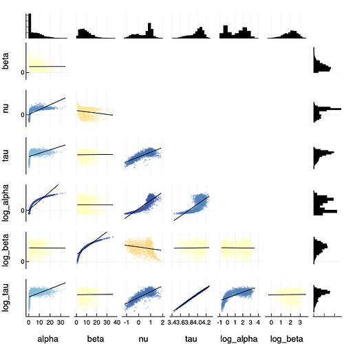
I think what you’re seeing here is a fundament nonidentifiabiltiy of the model. Data simulated from large alpha are able to excluded small alpha in the fit, and avoid the alpha/nu ridge, but data simulated from small alpha are consistent with both small alpha and large alpha which requires the fit into that nasty alpha/nu ridge. Look all of those lovely divergences!

Because the non-identifiability isn’t purely in the latent part of the model, there is no parameterization that will fix the problem. The only way forward is with informative priors that might be able to contain the fit into a region where the model is better identified, like we’ve done with Gaussian processes for certain kernels.

2 Likes

Isn’t 1 - Phi(x) = Phi(-x)? log(Phi(x)) could be replaced by normal_lcdf. That should be stable.

No, it is not. All of the log CDFS are currently implemented as the literal log of CDF functions and hence share the same numerical inaccuracy problems.

2 Likes

Thank you again for such a detailed explanation Mike!

My concern is that the original normal-halflaplace model I posted is much tighter around the true parameters when alpha is small than the new models with the better sampling behaviour are. Although of course these new models work better when alpha is big, and the old model works badly when alpha is big, the trouble with big alpha sort of made sense as Reed and Jorgenson say they have identification problems when alpha is big (because the model shouldn’t actually have the extra laplace tail in that case). So this situation with the new model is confusing to me, because it seems like the new improved model has trouble in the case that Reed and Jorgenson don’t have trouble.

Of course the original model (which had the Reed and Jorgenson type of trouble) also had much worse sampling behaviour in terms of divergences in all cases. But still, the posterior draws were much more closely clustered around the actual truth when alpha was small - and the results were appropriately responsive to changes in the generating alpha, so it’s not just that the prior was directing them to the region near zero or anything. So I am somewhat reluctant to adopt the new model in all cases – especially because in the application I’m considering I suspect alpha is in fact small.

Sure, but this was entirely due to the model fit not capturing the actual posterior. The new Stan programs are the same mathematically – the only difference are the more numerically robust implementations. In other words the results you saw in your initial Stan program weren’t the result of the model, but rather the results of the model marred by the numerical issues.

The old model appears to fit small alpha better only because the numerical issues coincidentally removed the parameter configurations far from the ground truth. Just like a broken clock is correct twice a day, a broken model will appear to be correct when the truth is far away from pathological neighborhoods.

I can’t comment on the Reed and Jorgenson results all that much, but one does have to be careful with the exact meaning of identification. If they’re referring to classic identifiability (likelihood converges to an increasingly smaller neighborhood around the truth as N increases) then that won’t necessarily be relevant here as the diffuse likelihood functions indication that such convergence would be really, really slow.

It may be worth exploring the practical identifiability (the shape of the likelihood function for finite N) more thorough to validate these results or not. In my cursory analyses the posterior predictive checks appeared to validate that the large alpha configurations predicted data entirely consistent with small alpha configurations which would be consistent with the weak identifiability. You can also compare the predictive distributions from different fits to see if there are any observable differences.

I wouldn’t be surprised if this model was indeed that weakly identified for finite N – trying to match tails is a notoriously hard problem.

1 Like