Differences in simplex constraining function vs normal simplex

Hey @WardBrian, I don’t think this was working as expected for me. As a simple example, this works:

parameters {
  simplex[J] beta;
}
model {
  beta ~ dirichlet(alpha);  // alpha defined elsewhere
}

but this doesn’t:

parameters {
  vector[J - 1] u;
}
transformed parameters {
  vector[J] beta = simplex_jacobian(u);
}
model {
  beta ~ dirichlet(alpha);  // alpha defined elsewhere
}

The manual says u is a free vector. Initially I was constraining u as follows, but this yields strange result and is also inconsistent with the documentation.

parameters {
  vector<lower=0, upper=1>[J - 1] u;
}

Could you please advise me where I’m going wrong?

Can you elaborate on what you mean by “doesn’t work”?

Hey Brian,

Sorry, that was super vague. Attached are traceplots. trace-beta.png are the traceplots for the simplex in the first configuration.

trace-u.png are the traceplots for the simplex for the second configuration, where beta = simplex_jacobian(u).

1 Like

I don’t have access to Stan atm. Can you set a seed when calling cmdstan and then tell us what the lp is when running flag = 0 and flag = 1?

data {
...
 int flag;
}
parameters {
  vector[J - 1] u;
}
transformed parameters {
  vector[J] beta;
}
model {
  if ( flag == 0 ) {
    beta = simplex_jacobian(u);
  } else {
    vector[J] beta_z = sum_to_zero_constrain(u);
    real r = log_sum_exp(z);
    target += 0.5 * log(N);
    target += sum(z) - N * r;
    beta = exp(z - r);
}
  beta ~ dirichlet(alpha);
}

Hey,

Don’t tell me I’ve using an older version of cmdstan!

I tweaked it to:

parameters {
  vector[J] beta;
  if (flag) {
    beta = simplex_jacobian(u);
  } else {
    vector[J] z = sum_to_zero_constrain(u);
    real r = log_sum_exp(z);
    jacobian += 0.5 * log(J);
    jacobian += sum(z) - J * r;
    beta = exp(z - r);
  }
}

And flag = 0 looks good. Here’s the output for lp__:

> map(fits, ~.$summary("lp__"))
[[1]]
# A tibble: 1 × 10
  variable  mean median    sd   mad    q5   q95  rhat ess_bulk ess_tail
  <chr>    <dbl>  <dbl> <dbl> <dbl> <dbl> <dbl> <dbl>    <dbl>    <dbl>
1 lp__     -569.  -567.  8.63  8.42 -584. -556.  1.02     210.     248.

[[2]]
# A tibble: 1 × 10
  variable  mean median    sd   mad    q5   q95  rhat ess_bulk ess_tail
  <chr>    <dbl>  <dbl> <dbl> <dbl> <dbl> <dbl> <dbl>    <dbl>    <dbl>
1 lp__     7178.  7178.  59.4  82.1 7084. 7263.  3.80     8.76     15.4
1 Like

What version are you using, out of curiosity?

This gives:

> cmdstan_version()
[1] "2.37.0"

And I did just install the development version, did install_cmdstan() again.

This seems to work for me

data {
 int<lower=1> J;
 vector[J] alpha;
 int flag;
}
parameters {
  vector[J - 1] u;
}
transformed parameters {
  vector[flag ? J : 0] beta_simplex_jacobian;
  vector[flag ? 0 : J] beta_simplex_manual;
  if (flag) {
    beta_simplex_jacobian = simplex_jacobian(u);
  } else {
    vector[J] z = sum_to_zero_constrain(u);
    real r = log_sum_exp(z);
    jacobian += 0.5 * log(J);
    jacobian += sum(z) - J * r;
    beta_simplex_manual = exp(z - r);
  }
}
model{
  if (flag) {
    beta_simplex_jacobian ~ dirichlet(alpha);
  } else {
    beta_simplex_manual  ~ dirichlet(alpha);
  }
}

R code

library(cmdstanr)

mod <- cmdstan_model(stan_file = "simplex.stan")

mod_out_manual <- mod$sample(
  data = list(flag = 0, J = 5, alpha = 1:5),
  seed = 2344,
  parallel_chains = 4,
  chains = 4
)
mod_out_jacobian <- mod$sample(
  data = list(flag = 1, J = 5, alpha = 1:5),
  seed = 2344,
  parallel_chains = 4,
  chains = 4
)

mod_out_jacobian$summary(c("lp__", "beta_simplex_jacobian"))
mod_out_manual$summary(c("lp__", "beta_simplex_manual"))

Output

> mod_out_jacobian$summary(c("lp__", "beta_simplex_jacobian"))
# A tibble: 6 × 10
  variable                     mean   median     sd    mad        q5     q95  rhat ess_bulk ess_tail
  <chr>                       <dbl>    <dbl>  <dbl>  <dbl>     <dbl>   <dbl> <dbl>    <dbl>    <dbl>
1 lp__                     -23.8    -23.4    1.51   1.37   -26.6     -22.0   1.00     1797.    2333.
2 beta_simplex_jacobian[1]   0.0656   0.0468 0.0627 0.0497   0.00314   0.190 1.000    2184.    1736.
3 beta_simplex_jacobian[2]   0.134    0.118  0.0863 0.0820   0.0247    0.295 1.00     3200.    1618.
4 beta_simplex_jacobian[3]   0.199    0.186  0.0984 0.0995   0.0613    0.380 1.00     3661.    2365.
5 beta_simplex_jacobian[4]   0.268    0.257  0.111  0.116    0.104     0.464 1.00     4181.    2834.
6 beta_simplex_jacobian[5]   0.334    0.326  0.117  0.120    0.152     0.539 1.00     3640.    2730.
> mod_out_manual$summary(c("lp__", "beta_simplex_manual"))
# A tibble: 6 × 10
  variable                   mean   median     sd    mad        q5     q95  rhat ess_bulk ess_tail
  <chr>                     <dbl>    <dbl>  <dbl>  <dbl>     <dbl>   <dbl> <dbl>    <dbl>    <dbl>
1 lp__                   -23.7    -23.3    1.50   1.30   -26.6     -21.9    1.00    1772.    2026.
2 beta_simplex_manual[1]   0.0686   0.0505 0.0629 0.0482   0.00391   0.195  1.00    2116.    1390.
3 beta_simplex_manual[2]   0.133    0.117  0.0842 0.0783   0.0280    0.300  1.00    3216.    2326.
4 beta_simplex_manual[3]   0.199    0.184  0.100  0.0977   0.0592    0.388  1.00    4080.    2258.
5 beta_simplex_manual[4]   0.267    0.254  0.112  0.117    0.104     0.465  1.00    3725.    2657.
6 beta_simplex_manual[5]   0.331    0.325  0.117  0.120    0.149     0.535  1.00    3098.    2468.

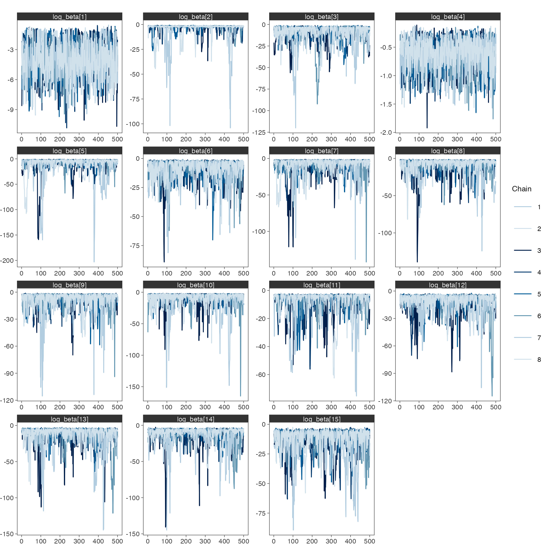
Thank you, that works for me as well. I think it’s coming down to the initial values, perhaps. Below is the Stan program I’m using it for, a Jolly-Seber mark-recapture model, with the definitions happening in transformed parameters. When I place a Dirichlet prior over beta with concentration parameters alpha, I get the horrible behaviour shown above. When I set alpha = ones_vector(J), mixing is much better but still horrible. So, I’m guessing the issue is that u is getting initialised and it’s yielding a horrible simplex beta. However, when I produce the simplex manually like you’ve done, the mixing is fine. So somewhere there’s a difference between the manual approach and the simplex_jacobian approach.

functions {
  #include ../stan/util.stanfunctions
  #include ../stan/js.stanfunctions
  #include ../stan/js-rng.stanfunctions
}

data {
  int<lower=1> I, J;  // number of individuals and surveys
  vector<lower=0>[J - 1] tau;  // survey intervals
  array[I, J] int<lower=0, upper=1> y;  // detection history
  int<lower=1> I_aug;  // number of augmented individuals
  int<lower=0, upper=1> dir,  // logistic-normal (0) or Dirichlet (1) entry
                        intervals;  // ignore intervals (0) or not (1)
}

transformed data {
  int I_all = I + I_aug, Jm1 = J - 1;
  array[I, 2] int f_l = first_last(y);
  vector[Jm1] tau_scl = tau / mean(tau), log_tau_scl = log(tau_scl);
}

parameters {
  real<lower=0> h;  // mortality hazard rate
  vector<lower=0, upper=1>[J] p;  // detection probabilities
  real<lower=0> mu;  // concentration parameters or logistic-normal scale
  vector[Jm1] u;  // unconstrained entries
  real<lower=0, upper=1> psi;  // inclusion probability
}

transformed parameters {
  vector[J] log_alpha = dir ? 
                        rep_vector(log(mu), J) 
                        : append_row(0, mu * u);
  if (intervals) {
    log_alpha[2:] += log_tau_scl;
  }

  // this approach doesn't work well
  vector[J] log_beta = dir ?
                       log(simplex_jacobian(u))
                       : log_softmax(log_alpha);

  // this works well
  vector[J] log_beta;
  if (dir) {
    vector[J] z = sum_to_zero_constrain(u);
    real r = log_sum_exp(z);
    log_beta = z - r;
    jacobian += 0.5 * log(J);
    jacobian += sum(z) - J * r;
  } else {
    log_beta = log_softmax(log_alpha);
  }
  real lprior = gamma_lpdf(h | 1, 3) + beta_lpdf(p | 1, 1) 
                + gamma_lpdf(mu | 1, 1); 
}

model {
  vector[Jm1] log_phi = -h * tau;
  vector[J] logit_p = logit(p);
  tuple(vector[I], vector[2], matrix[J, I], vector[J]) lp =
    js(y, f_l, log_phi, logit_p, log_beta, psi);
  target += sum(lp.1) + I_aug * log_sum_exp(lp.2);
  target += lprior;
  target += dir ? 
            dirichlet_lupdf(exp(log_beta) | exp(log_alpha))  // ones_vector(J) works OK
            : std_normal_lupdf(u);
}

generated quantities {
  vector[I] log_lik;
  array[J] int N, B, D;
  int N_super;
  {
    vector[Jm1] log_phi = -h * tau;
    vector[J] logit_p = logit(p);
    tuple(vector[I], vector[2], matrix[J, I], vector[J]) lp =
      js(y, f_l, log_phi, logit_p, log_beta, psi);
    log_lik = lp.1;
    tuple(array[J] int, array[J] int, array[J] int, int) latent =
      js_rng(lp, f_l, log_phi, logit_p, I_aug);
    N = latent.1;
    B = latent.2;
    D = latent.3;
    N_super = latent.4;
  }
}

Can you test this? I think it’s the same as the Stan-math cpp code

functions {
  // Transform a (K-1)-vector y to a K-simplex using the ILR-based
  // construction with an online softmax for numerical stability.
  //
  // This is equivalent (up to numerical details) to
  //   softmax(sum_to_zero_constrain(y))
  // and adds the corresponding log-Jacobian contribution to target.
  //
  // Input:  y (dimension K-1)
  // Output: simplex (dimension K)
  vector simplex_cpp_jacobian(vector y) {
    int N = num_elements(y);    // N = K - 1
    int K = N + 1;              // simplex dimension
    vector[K] z;
    real sum_w;
    real d;
    real max_val;
    real max_val_old;

    // Initialize
    z = rep_vector(0.0, K);

    // Degenerate case K = 1 (N = 0): simplex is just [1]
    if (N == 0) {
      z[1] = 1.0;
      return z;
    }

    sum_w      = 0.0;
    d          = 0.0;                 // running sum of exponentials
    max_val    = 0.0;
    max_val_old = negative_infinity();

    // Main loop: i = N, N-1, ..., 1
    for (k in 1:N) {
      int i = N + 1 - k;         // maps offset=1→i=N, ..., offset=N→i=1
      real n = i;
      real w = y[i] / sqrt(n * (n + 1));

      sum_w += w;

      // z_raw updates (pre-softmax scores)
      z[i]     += sum_w;
      z[i + 1] -= w * n;

      // Online log-sum-exp update on z[i+1]
      max_val = fmax(max_val_old, z[i + 1]);
      d = d * exp(max_val_old - max_val) + exp(z[i + 1] - max_val);
      max_val_old = max_val;
    }

    // Include z[1] in the log-sum-exp accumulation
    max_val = fmax(max_val_old, z[1]);
    d = d * exp(max_val_old - max_val) + exp(z[1] - max_val);
    z = exp(z - max_val) / d;
    // Final softmax normalization: z := softmax(z_raw)

    // Jacobian contribution:
    // lp += sum(log(z)) + 0.5 * log(K)
    // but sum(log(z)) = -K * (max_val + log d)
    jacobian += -K * (max_val + log(d)) + 0.5 * log(K);

    return z;
  }
}

This one samples well!

Umm…I’m not sure then. Maybe the rev speciality @WardBrian?

I can investigate this week, but it seems like it must be something pretty weird, since the simplex type is using the same function and rev specialization under the hood…

1 Like

@mhollanders can you try splitting the log() up? I wonder if something weird is happening with the jacobian adjustment and the log function. Something like:

 // this approach doesn't work well
  vector[J] beta = simplex_jacobian(u);
  vector[J] log_beta = log(beta);

Another thing to check in the code that “doesn’t work” try adding a dummy call to jacobian to the code, i.e.,

jacobian += 0;

The stanc3 generation may have a bug where it’s doing the old style. Possibly when a constraint function with _jacobian is wrapped in a function call and there’s no additional jacobian += to add the log-det-jacobian adjustment.

I can’t explain why but the model is working now. I literally copy-and-pasted the previously posted code, (un)commented the required sections, and it’s running fine. Sorry about this, I have no idea what happened or how to even recreate the wonky traceplots from before.

functions {
  #include ../stan/util.stanfunctions
  #include ../stan/js.stanfunctions
  #include ../stan/js-rng.stanfunctions
}

data {
  int<lower=1> I, J;  // number of individuals and surveys
  vector<lower=0>[J - 1] tau;  // survey intervals
  array[I, J] int<lower=0, upper=1> y;  // detection history
  int<lower=1> I_aug;  // number of augmented individuals
  int<lower=0, upper=1> dir,  // logistic-normal (0) or Dirichlet (1) entry
                        intervals;  // ignore intervals (0) or not (1)
}

transformed data {
  int I_all = I + I_aug, Jm1 = J - 1;
  array[I, 2] int f_l = first_last(y);
  vector[Jm1] tau_scl = tau / mean(tau), log_tau_scl = log(tau_scl);
}

parameters {
  real<lower=0> h;  // mortality hazard rate
  vector<lower=0, upper=1>[J] p;  // detection probabilities
  real<lower=0> mu;  // concentration parameters or logistic-normal scale
  vector[Jm1] u;  // unconstrained entries
  real<lower=0, upper=1> psi;  // inclusion probability
}

transformed parameters {
  vector[J] log_alpha = dir ? 
                        rep_vector(log(mu), J) 
                        : append_row(0, mu * u);
  if (intervals) {
    log_alpha[2:] += log_tau_scl;
  }

  // this approach doesn't work well
  vector[J] log_beta = dir ?
                       log(simplex_jacobian(u))
                       : log_softmax(log_alpha);

  // this works well
  vector[J] log_beta;
  if (dir) {
    vector[J] z = sum_to_zero_constrain(u);
    real r = log_sum_exp(z);
    log_beta = z - r;
    jacobian += 0.5 * log(J);
    jacobian += sum(z) - J * r;
  } else {
    log_beta = log_softmax(log_alpha);
  }
  real lprior = gamma_lpdf(h | 1, 3) + beta_lpdf(p | 1, 1) 
                + gamma_lpdf(mu | 1, 1); 
}

model {
  vector[Jm1] log_phi = -h * tau;
  vector[J] logit_p = logit(p);
  tuple(vector[I], vector[2], matrix[J, I], vector[J]) lp =
    js(y, f_l, log_phi, logit_p, log_beta, psi);
  target += sum(lp.1) + I_aug * log_sum_exp(lp.2);
  target += lprior;
  target += dir ? 
            dirichlet_lupdf(exp(log_beta) | exp(log_alpha))  // ones_vector(J) works OK
            : std_normal_lupdf(u);
}

generated quantities {
  vector[I] log_lik;
  array[J] int N, B, D;
  int N_super;
  {
    vector[Jm1] log_phi = -h * tau;
    vector[J] logit_p = logit(p);
    tuple(vector[I], vector[2], matrix[J, I], vector[J]) lp =
      js(y, f_l, log_phi, logit_p, log_beta, psi);
    log_lik = lp.1;
    tuple(array[J] int, array[J] int, array[J] int, int) latent =
      js_rng(lp, f_l, log_phi, logit_p, I_aug);
    N = latent.1;
    B = latent.2;
    D = latent.3;
    N_super = latent.4;
  }
}

Hey - a solved problem is a solved problem!

Out of curiosity, were you running all these experiments in the same file? Is it possible that a different compiled version was left around on disk, like maybe the version you tried putting an upper and lower bound on u? I wouldn’t be shocked if that version sampled poorly

I kept saving new .stan files so I don’t think that was it. Originally, I hadn’t noticed this behaviour because I thought u had to be constrained between 0 and 1 before simplex constraining, and I noticed the issue when I declared u to be an unconstarined vector. If it pops up again, I’ll let you know.

Great!

I’ll send you the bill :)

3 Likes

Sorry to rehash this but I just want to flag I’m still getting similar issues. Without showing the whole model, this Stan program mixes well:

parameters {
  simplex[V[1]] phi_psi;
  simplex[V[2]] phi_mu;
}
transformed parameters {
  // ragged matrix of simplexes
  matrix[2, V[2]] phi = rep_matrix(0, 2, V[2]);
  phi[1, :V[1]] = phi_psi';
  phi[2] = phi_mu';
}

and this one doesn’t.

parameters {
  vector[sum(V) - 2] phi_u;
}
transformed parameters {
  matrix[2, V[2]] phi = rep_matrix(0, 2, V[2]);
  phi[1, :V[1]] = simplex_jacobian(head(phi_u, V[1] - 1))';
  phi[2] = simplex_jacobian(tail(phi_u, V[2] - 1))';
}

I’m pretty sure it’s due to initial values but I could be wrong. The reason I think so is as you can see in previous posts, I have had decent runs. But it’s unreliable and when I go back manually putting in the simplexes it’s fine.

Cheers,

Matt