Convergence Troubles and Pathologies in an already Reparameterized Model

Hi all,

I’ve been bashing my head against the wall for several months now trying to figure out this problem, and now hope to turn to you, Stan Community, for some insights. I will give the mathematical formulation to the model first, which you are welcome to read for a bit of background. Then I will give the Stan code, followed by some of the convergence issues and pathologies that I have been running into.


Mathematical Model Description

I would like to fit the following model in Stan:

Y \sim Multinomial(\Pi)
\pi_k = \dfrac{u(r_k) - u(r_{k-1})}{u(r_K)} , for k \in 2...K, and \pi_1 = 1-\sum_2^K \pi_k

Here, we have bird count data that is separated into K distance bands, with each band having a maximum radius of r_k. The function u(r) = 1 - \exp\left(-\dfrac{r^2}{\tau_s^2}\right) , where \tau is an effective detection radius for species s, and can be modelled as follows:
\log(\tau_s) \sim N(\mu_s, \sigma)
\mu_s = \alpha + MIG_s + HAB_s + \beta_1 \times MASS_s + \beta_2 \times PITCH_s
\alpha \sim N(4,0.1)
MIG, HAB \sim N(0, 0.05)
\beta_1 \sim N(0.01, 0.005)
\beta_2 \sim N(-0.01, 0.005)
\sigma \sim \exp(5)

In plain terms, I am modelling a species’ effective detection radius as a function of the species’ migratory status (2 factors), habitat preference (2 factors), mass (log scaled and centred), and song pitch (scaled and centred). I have data for 300+ species, with anywhere between 5 and 90,000 data points per species. The priors imply that an “average” effective detection radius would be around 54.6m (i.e., exp(4)), with that changing based on migratory status and habitat preference, increasing with increased mass, but decreasing with increasing pitch. The prior predictive checks for this model look excellent.


Stan Model Code

functions {
  real partial_sum_lpmf(array[, ] int slice_abund_per_band, // modifications to avoid Stan warnings at compile
                        int start, int end,
                        int max_intervals,
                        array[] int bands_per_sample,
                        array[, ] real max_dist,
                        array[] int species,
                        vector log_tau)
  {
    real lp = 0;
    int Pi_size = end - start + 1;
    int Pi_index = 1;
    matrix[Pi_size, max_intervals] Pi = rep_matrix(0, Pi_size, max_intervals);
    
    for (i in start:end)
    {
      for (k in 1:(bands_per_sample[i]-1)) // what if the final band was usedas the constraint? more effecient?
      {
        if(k > 1){
        Pi[Pi_index,k] = ((1 - exp(-(max_dist[i,k]^2 / exp(log_tau[species[i]])^2))) - 
        (1 - exp(-(max_dist[i,k - 1]^2 / exp(log_tau[species[i]])^2)))) / 
        (1 - exp(-(max_dist[i,bands_per_sample[i]]^2 / exp(log_tau[species[i]])^2)));
        }else{
        Pi[Pi_index,k] = (1 - exp(-(max_dist[i,k]^2 / exp(log_tau[species[i]])^2))) /
        (1 - exp(-(max_dist[i,bands_per_sample[i]]^2 / exp(log_tau[species[i]])^2)));
        }
      }
      Pi[Pi_index,bands_per_sample[i]] = 1 - sum(Pi[Pi_index,]); // what if the final band was used as the constraint?
      
      lp = lp + multinomial_lpmf(slice_abund_per_band[Pi_index, ] | to_vector(Pi[Pi_index, ]));
      Pi_index = Pi_index + 1;
     
    }
    
    return lp;
  }

}

data {
  int<lower = 1> n_samples;           // total number of sampling events i
  int<lower = 1> n_species;           // total number of specise
  int<lower = 2> max_intervals;       // maximum number of intervals being considered
  int<lower = 1> grainsize;           // grainsize for reduce_sum() function
  array[n_samples] int species;             // species being considered for each sample
  array[n_samples, max_intervals] int abund_per_band;// abundance in distance band k for sample i
  array[n_samples] int bands_per_sample; // number of distance bands for sample i
  array[n_samples, max_intervals] real max_dist; // max distance for distance band k
  int<lower = 1> n_mig_strat;        //total number of migration strategies
  array[n_species] int mig_strat;        //migration strategy for each species
  int<lower = 1> n_habitat;        //total number of habitat preferences
  array[n_species] int habitat;        //habitat preference for each species
  array[n_species] real mass;  //log mass of species
  array[n_species] real pitch; //song pitch of species
}

parameters {
  real mu_mig_strat_raw;
  real mu_habitat_raw;
  real beta_mass_raw;
  real beta_pitch_raw;
  real<lower = 0> sigma;
  vector[n_species] log_tau_raw;
}

transformed parameters {
  row_vector[n_species] mu;
  row_vector[n_mig_strat] mu_mig_strat;
  row_vector[n_habitat] mu_habitat;
  real beta_mass;
  real beta_pitch;
  vector[n_species] log_tau;
  
  mu_mig_strat[1] = 0; //fixing one of the intercepts at 0
  mu_habitat[1] = 0; //fixing one of the intercepts at 0
  mu_mig_strat[2] = mu_mig_strat_raw * 0.05; 
  mu_habitat[2] = mu_habitat_raw * 0.05;
  beta_mass = 0.01 + (0.005 * beta_mass_raw); # small positive slope
  beta_pitch = -0.01 + (0.005 * beta_pitch_raw); # small negative slope
  
  for (sp in 1:n_species)
  {
    mu[sp] = mu_mig_strat[mig_strat[sp]] +
                       mu_habitat[habitat[sp]] + //should this be the habitat at the survey?
                       beta_mass * mass[sp] +
                       beta_pitch * pitch[sp];
                       
    log_tau[sp] = mu[sp] + (log_tau_raw[sp] * sigma);
  }
}

model {
  log_tau_raw ~ std_normal();
  mu_mig_strat_raw ~ std_normal();
  mu_habitat_raw ~ std_normal();
  beta_mass_raw ~ std_normal();
  beta_pitch_raw ~ std_normal();
  
  sigma ~ exponential(5);

  target += reduce_sum(partial_sum_lpmf,
                       abund_per_band,
                       grainsize,
                       max_intervals,
                       bands_per_sample,
                       max_dist,
                       species,
                       log_tau);
                       

}


Convergence Issues and Pathologies
Okay, so I have had nothing but issues with this model, and I just am not sure how to rethink this model. When running all species with all data, the model takes a LONG time to run (3 or so weeks). Half of the parameters are poorly converged (Rhat > 1.1), and most of the parameters have very low ESS (<100). A similarly sized model (size as in number of species and number of data points) that I built in Stan (albeit with far fewer parameters) took less than 24 hours to run.

In an attempt to start doing some diagnosing, I went ahead and moved down to a simpler model, that only considers 1 species and just tries to model the mean EDR for that species. I.e., nothing affecting EDR. I got some really bizarre shapes to some of the pair plots. Some examples:


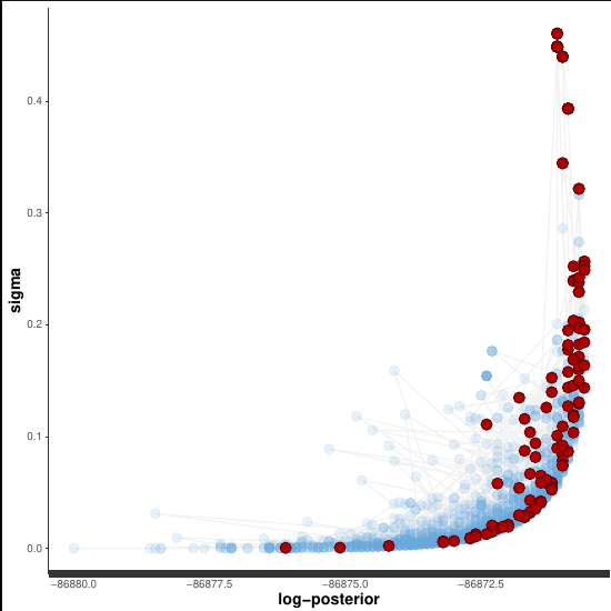
This of course makes me think of the Neal’s funnel example, where one of the fixes is to sample from the standard normal distribution and transform the parameters in the transformed parameters block. But, that’s what I already do! In fact I’ve tried my best to take great care to make this as efficient of a sampling space as possible, given the model.

I wonder if anyone here can provide any suggestions of what I might be missing?

Happy to provide any more additional information as needed.

Thanks!
Brandon

1 Like

With between 5 and 90000 data points per species, you might try centering the strongly informed species and non-centering the weakly informed species. I’m guessing–but tell me if I’m wrong–that when you moved down to one species you remained in the non-centered parameterization but chose one of the very strongly informed species. What happens if you:

  • fit a 1-species example with one of the weakly informed species
  • fit a multispecies example with multiple weakly informed species (say fewer than 50 data points per species)
  • fit a 1-species model in the centered parameterization with a strongly informed species

Thanks for the reply! I hadn’t thought of having a mixture of centring and non-centring, and to be honest did not expect the number of data points to make a difference based on if the model is centred or non-centred. I went through your suggestions here and added some of my own trials, results as follows:

  • fit a 1-species example with one of the weakly informed species, non-centred: WORKS FINE
  • fit a multispecies example with multiple weakly informed species, non-centred: WORKS FINE
  • fit a 1-species model in the centred parameterization with a strong informed species: WORKS 😲

I also then tried the following:

  • fit a multispecies example with multiple weakly informed species, with a centred parameterization: DID NOT WORK WELL (many divergences)
  • fit a 1-species example with one of the weakly informed species, centred parameterization: WORKS FINE

I did not try a multispecies model with multiple strongly informed species in the centred parameterization yet. But I am getting the sense that this mixture of centred and non-centred parameterization might be a thought worth pursuing.

So, in order to fit a model with a mixture of a parameterizations, this is my thought of how to do it:

  • make a rule of minimum sample size to have a centred parameterization (e.g., 50, 100, 200?)
  • make a vector of species that fall below the minimum sample size, and a vector of species that fall above the minimum sample size
  • in the stan model, iterate through the vector of species below minimum sample size in the transformed parameters block, and sample using non-centred parameterization
  • also in the stan model, iterate through the vector of species above the minimum sample size in the model block, and sample using centred parameterization

Would something like that make sense?

Thanks again!

1 Like

Yep, that sounds right :)

Hi again!

First off, thanks for your help in pointing me toward the mixed parameterizations. I ended up reading Michael Betancourt’s post on Hierarchical Modelling which I found super informative.

Unfortunately, unless I’ve done something wrong in reparameterizing my model, this does not seem to be doing the trick. I have posted the model code below, which is based off Michael Betancourt’s example here. I tested the model on a few of the scenarios you had listed above, and got a few divergences, with slow sampling. I’ve been running the “full” model with all species and data points since July 19th (today is the 27th), and it is only halfway through warmup (500/1000 warmup iterations, with 2000 sampling iterations still to go). So, I think I will likely pull the plug on that model run.

Here is the model that I wrote for the mixed parameterization. I wonder if there is something I have missed here? I note too that it is only the log_tau parameter that is being considered for the mixed parameterization, I’m sure the other parameters (e.g., intercept, mu_mig_strat, beta_mass, etc.) do not need to be considered? Or do they?

functions {
  real partial_sum_lpmf(array[, ] int slice_abund_per_band, // modifications to avoid Stan warnings at compile
                        int start, int end,
                        int max_intervals,
                        array[] int bands_per_sample,
                        array[, ] real max_dist,
                        array[] int species,
                        vector log_tau)
  {
    real lp = 0;
    int Pi_size = end - start + 1;
    int Pi_index = 1;
    matrix[Pi_size, max_intervals] Pi = rep_matrix(0, Pi_size, max_intervals);
    
    for (i in start:end)
    {
      for (k in 1:(bands_per_sample[i]-1)) // what if the final band was usedas the constraint? more effecient?
      {
        if(k > 1){
        Pi[Pi_index,k] = ((1 - exp(-(max_dist[i,k]^2 / exp(log_tau[species[i]]^2)))) - 
        (1 - exp(-(max_dist[i,k - 1]^2 / exp(log_tau[species[i]]^2))))) / 
        (1 - exp(-(max_dist[i,bands_per_sample[i]]^2 / exp(log_tau[species[i]]^2))));
        }else{
        Pi[Pi_index,k] = (1 - exp(-(max_dist[i,k]^2 / exp(log_tau[species[i]]^2)))) /
        (1 - exp(-(max_dist[i,bands_per_sample[i]]^2 / exp(log_tau[species[i]]^2))));
        }
      }
      Pi[Pi_index,bands_per_sample[i]] = 1 - sum(Pi[Pi_index,]); // what if the final band was used as the constraint?
      
      lp = lp + multinomial_lpmf(slice_abund_per_band[Pi_index, ] | to_vector(Pi[Pi_index, ]));
      Pi_index = Pi_index + 1;
     
    }
    
    return lp;
  }

}

data {
  int<lower = 1> n_samples;           // total number of sampling events i
  int<lower = 2> max_intervals;       // maximum number of intervals being considered
  array[n_samples, max_intervals] int abund_per_band;// abundance in distance band k for sample i
  array[n_samples] int bands_per_sample; // number of distance bands for sample i
  array[n_samples, max_intervals] real max_dist; // max distance for distance band k
  
  int<lower = 1> n_species;           // total number of species
  array[n_samples] int species;       // species being considered for each sample
  
  int<lower = 1> n_species_ncp;     // how many non-centred species to model
  array[n_species_ncp] int species_ncp;  // vector of indices corresponding to non-centred species
  
  int<lower = 1> n_species_cp;        // how many centred species to model
  array[n_species_cp] int species_cp;       // vector of indices correspondnig to centred species

  int<lower = 1> n_mig_strat;        //total number of migration strategies
  array[n_species] int mig_strat;        //migration strategy for each species
  
  int<lower = 1> n_habitat;        //total number of habitat preferences
  array[n_species] int habitat;        //habitat preference for each species
  
  array[n_species] real mass;  //log mass of species
  
  array[n_species] real pitch; //song pitch of species

  int<lower = 1> grainsize;           // grainsize for reduce_sum() function
}

parameters {
  real intercept;
  row_vector[n_mig_strat] mu_mig_strat;
  row_vector[n_habitat] mu_habitat;
  real beta_mass;
  real beta_pitch;
  real<lower = 0> sigma;
  
  vector[n_species_ncp] log_tau_ncp; // non-centred species log tau
  vector[n_species_cp] log_tau_cp; // centred species log tau
}

transformed parameters {
  vector[n_species] mu;
  vector[n_species] log_tau;
  
  for (sp in 1:n_species)
  {
    mu[sp] = intercept + mu_mig_strat[mig_strat[sp]] +
                       mu_habitat[habitat[sp]] + 
                       beta_mass * mass[sp] +
                       beta_pitch * pitch[sp];
  }
  
  log_tau[species_ncp] = mu[species_ncp] + sigma * log_tau_ncp;
  log_tau[species_cp] = log_tau_cp;
}

model {
  intercept ~ normal(0.05, 0.1);
  mu_mig_strat ~ normal(0,0.05);
  mu_habitat ~ normal(0,0.05);
  beta_mass ~ normal(0.01,0.005);
  beta_pitch ~ normal(0.01,0.005);
  
  sigma ~ exponential(5);
  
  log_tau_ncp ~ std_normal();
  log_tau_cp ~ normal(mu[species_cp], sigma);

  target += reduce_sum(partial_sum_lpmf,
                       abund_per_band,
                       grainsize,
                       max_intervals,
                       bands_per_sample,
                       max_dist,
                       species,
                       log_tau);
}

Thanks!

Brandon

That code looks a bit off. Before you had

  1 - exp(-(max_dist[i,k]^2 / exp(log_tau[species[i]])^2))

but now you have

  1 - exp(-(max_dist[i,k]^2 / exp(log_tau[species[i]]^2)))

and squaring log_tau does not really make sense–it’s tau that’s squared in the model. Maybe you were thinking of

  1 - exp(-(max_dist[i,k]^2 / exp(log_tau[species[i]]*2)))

Simplifying the expressions should speed things up a bit. This should be equivalent to the first function but with fewer operations.

  real partial_sum_lpmf(array[, ] int slice_abund_per_band,
                        int start, int end,
                        int max_intervals,
                        array[] int bands_per_sample,
                        array[, ] real max_dist,
                        array[] int species,
                        vector log_tau)
  {
    int Pi_size = end - start + 1;
    int Pi_index = 1;
    array[Pi_size] real lps;
    for (i in start:end)
    {
      int n_max = bands_per_sample[i];
      real neg_inv_tau = -exp(-2*log_tau[species[i]]);
      vector[n_max] Ri = exp(neg_inv_tau * square(to_vector(max_dist[i])));
      real C = inv(1 - Ri[n_max]);
      vector[n_max] Pi;
      Pi[1] = C*(1 - Ri[1]);
      for (k in 2 : n_max) {
        Pi[k] = C*(Ri[k-1] - Ri[k]);
      }
      lps[Pi_index] = multinomial_lupmf(slice_abund_per_band[Pi_index, 1:n_max] | Pi);
      Pi_index = Pi_index + 1;
    }
    
    return sum(lps);
  }

I changed multinomial_lpmf to multinomial_lupmf because the normalizing constant is unnecessary but could be expensive to compute. To take advantage of that _lupmf form must be used with reduce_sum() as well.

  target += reduce_sum(partial_sum_lupmf,
                       abund_per_band,
                       grainsize,
                       max_intervals,
                       bands_per_sample,
                       max_dist,
                       species,
                       log_tau);
1 Like