Consistent errors (bias) in retrodiction/parameter recovery of a single parameter in a multilevel gamma model

The Short Story
I have written a multilevel model that includes normal and gamma distributions, and it does really well at retrodicting (i.e. recovering) the “true” parameters from simulated data. However, for one parameter is does a bad job at retrodiction. No matter what the true parameters are in the simulated data, the estimator is too high. This is not a result of overinformative priors, nor the result of lower-level estimators. Therefore, there is some kind of “bias” or consistent error in my Bayesian estimator, and I don’t know how to approach fixing it. I would love some help or references to literature on the subject to try to resolve this. Thank you!

The Longer Story
I am looking at the calls that individual frogs in a population make to understand how they are distributed for an evolutionary model. Each frog has a repertoire—a normal distribution of frequencies—which is parameterized by a peak frequency (the mean of the normal distribution, \overline x) and a repretoire width (the standard deviation of the normal distribution, s). I am trying to derive parameters that describe the population’s distribution of repertoire parameters. If the model were very simple, this would be the mean and standard deviation of each of the peak and width of frog repertoires (i.e. a bivariate normal distribution). However, because s must be positive, we have to use gamma distributions in the place of normal distributions, and this makes life a bit harder.

I have the following model:
x_i\sim\mathcal N(\overline x_{\textrm{frog}[i]}, s_{\textrm{frog}[i]}) // The calls produced by a frog follow that frog’s inherent normal distribution
\overline x_j\sim\mathcal N(\mu, \sigma) // The peak frequencies of frog repertoires in the population follows a normal distribution with a mean \mu and standard deviation \sigma
s_j\sim\mathcal G(\gamma, \gamma/\nu) // The widths of frog repertoires in the population follow a gamma distribution with shape \gamma and rate \gamma/\nu — the mean of this distribution is \nu, and the standard deviation of this distribution is \nu/\sqrt{\gamma}.

The main issue I’m facing is that the model retrodicts \gamma incredibly well, but totally whiffs it for \nu. Here’s a plot of the posteriors for each population (all populations are fit independently in a single MCMC run).


And as I move the true values of \nu that go into the simulated data, the posteriors move so that they are just too far right of the “true” values.

What’s strange is that it also does really well for s, which is the “data” that goes into fitting \nu and \gamma:


I suppose on some level this makes sense, because \gamma would not be fit well if s were not fitting well.

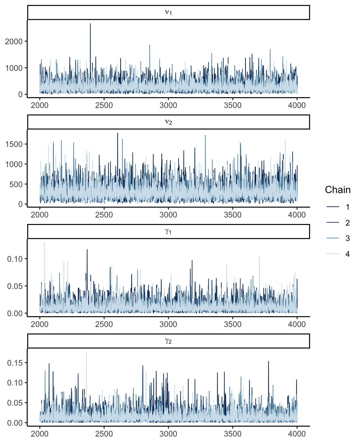
The traceplots look good:


And the density overlays are all similar:

Autocorrelation seems weirdly high in \mu and \sigma (which is concerning), but for \nu which actually faces tangible fitting problems, and for \gamma, autocorrelation drops off quickly:

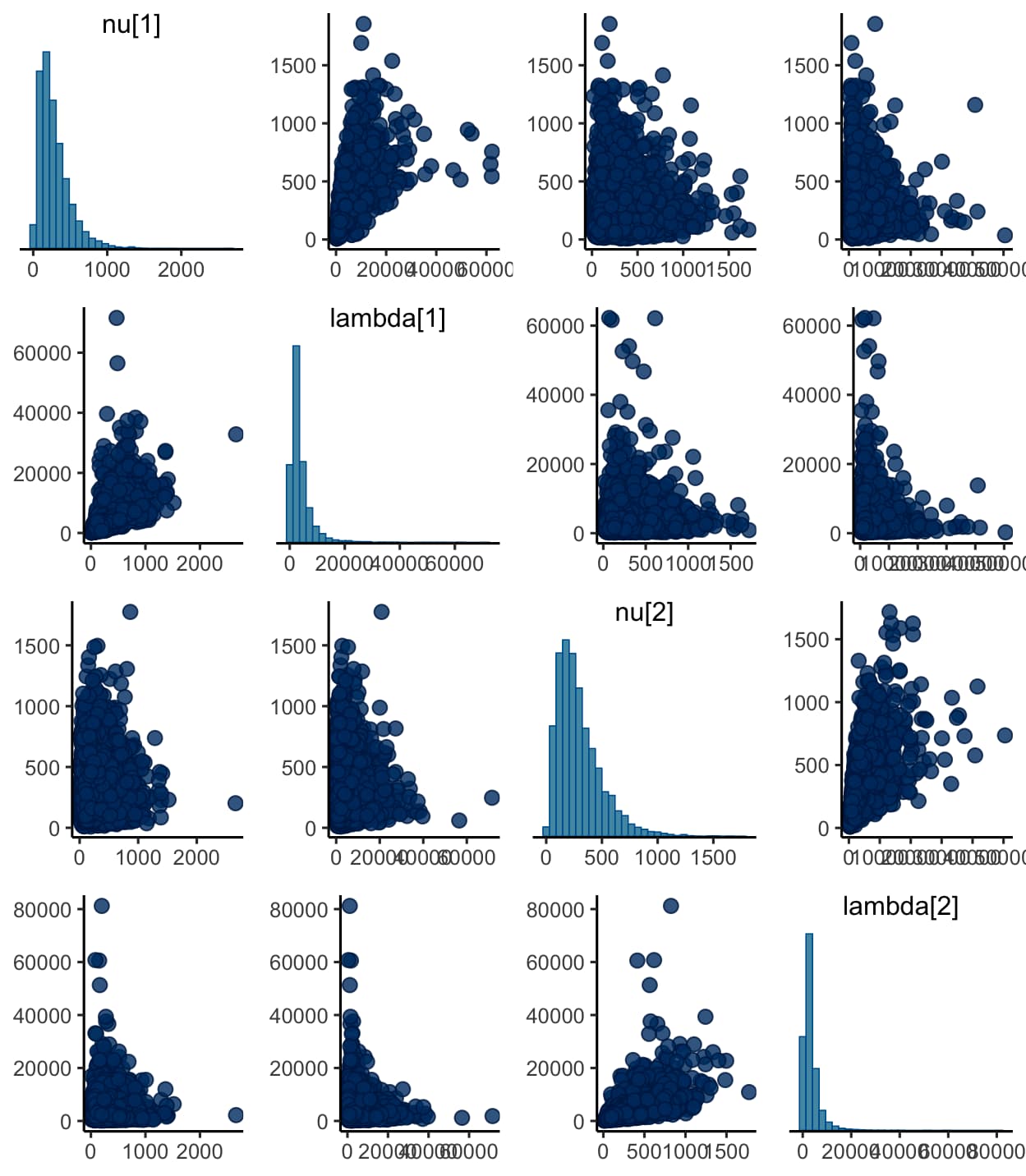
A pairwise correlation plot for each variable shows that each parameter is explored independently of all others.

I wondered if this was happening because s of \gamma were too low at the beginning of the chains, and thus this was causing \textbf P(\nu|\gamma, s)\propto\exp(-\gamma s/\nu) values too be too high for larger values of \nu. So I ran my chains for 6k iterations with 3k warmup, and it didn’t change anything.

In case it makes a difference, I’m running my analyses with adapt_delta=0.975 and max_treedepth=12. Thank you in advance for any of your ideas! And I’m happy to include any more information you’d like as well.

data {
  int nCall; // number of calls
  int nFrog; // number of frogs
  int nPopulation; // number of populations
  array[nCall] int frog; // group indicator for frogs
  array[nFrog] int population; // group indicator for populations
  vector[nCall] x; // peak frequency of each call
}

parameters {
  vector[nPopulation] mu; // Population average of peak
  vector<lower=0>[nPopulation] sigma; // Population std of peak
  vector<lower=0>[nPopulation] nu;  // Population average of width
  vector<lower=0>[nPopulation] gamma; // Population std of width

  vector[nFrog] xbar_raw; // Frog peaks
  vector<lower=0>[nFrog] s; // Frog widths
}

transformed parameters {
  vector[nFrog] xbar;
  for (j in 1:nFrog)
    xbar[j] = mu[population[j]] + sigma[population[j]] * xbar_raw[j]; // Non-centered parameterization of xbar
}

model {
  // Population-level parameters
  mu ~ normal(4500, 300);
  sigma ~ gamma(4, 0.01);  // mean = 400, std dev = 200
  nu ~ gamma(1.56, 0.006); // mean = 275, std dev = 225
  gamma ~ gamma(1.6, 0.5); // gives lambda = nu/sqrt(gamma)
                           // mean 200 and std dev 100

  // Individual-level parameters
  xbar_raw ~ normal(0, 1);
  for (j in 1:nFrog)
    s[j] ~ gamma(gamma[population[j]], gamma[population[j]]/nu[population[j]]);

  // Call-level likelihood
  x ~ normal(xbar[frog], s[frog]);
}

generated quantities {
  vector[nPopulation] lambda;
  for (k in 1:nPopulation)
    lambda[k] = nu[k]/sqrt(gamma[k]); // The standard deviation of s ~ gamma(gamma, gamma/nu)
}

Can you see if one of the alternative gamma distribution parameterizations solves this? The alternatives are at Add orthogonal parameterization of gamma distribution · Issue #3040 · stan-dev/math · GitHub. It would be good to know if these fix this issue because we can add it to the list.

1 Like

Hi spinkney,

Thank you for the excellent resources! I understand much better why I am having problems (and in particular why \gamma's doing well means that \nu suffers). I really appreciate how supportive this community is, especially to new members such as myself.

Firstly: I was looking at the Johnny gamma parameterization, which looks really exciting. In your implementation you have the function johnnys_gamma_lpdf(vector x, real tau, vector mu) have signature vector, real, vector.

I am using the function in my model section as:

for (j in 1:nFrog)
    s[j] ~ johnnys_gamma(gamma[population[j]], nu[population[j]]);

So that each frog has a repertoire width that follows a Gamma distribution with parameters specific to that frog’s parent population (populations are completely independent, with no partial pooling). (For clarity, my \gamma is Johnny’s \tau and my \nu is Johnny’s \mu.) Stan seems to get upset at this because s[j] is real and not a vector as it expects. I am woefully unqualified to make any edits to the function, or to even know the nuance of why Stan marks this as an error. (I did try changing vector x to be real x and it caused a whole chain of errors.) Do you have any ideas about how to approach fixing this? Or is this just the wrong parameterization for my problem?

Looking back at Johnny’s original post, it looks like I should be able to use:

real jgamma_lpdf(real x, real tau, real mu) {
  return (tau-1)*log(x)+tau*(log(tau)-log(mu)-lgamma(tau))-x*tau/mu;
 }

In my model as:

for (j in 1:nFrog)
    s[j] ~ jgamma(gamma[population[j]], nu[population[j]]);

(It claims it will run, but after dinner I’ll check back in with more info there.)

Secondly: I could be very wrong, but in the Mantei parameterization, it looks like Mantei’s \phi^{-1}=\gamma and Mantei’s \mu=\nu, and other than those variable names changing, this is actually the same model. Or, at the very least, I don’t know what I would change between the two! I’m using the gamma(—, —/mean) parameterization, and it looks like that’s the same form as Mantei’s formulation. (I’ll also double-check this after dinner, because I have a feeling I’m missing something here.)

Thank you!

I’ve managed to trade one problem for another. Using the jgamma function from above, I now perfectly retrodict \nu, but the \gamma estimate is worthless (thought it also runs faster now, which is kind of fun). Here’s the plot:

From the traceplots it appears that the NUTS doesn’t sample above values close to 0, which is a problem because we need it to find values as high as 2 or 3 (to be sure that all reasonable values will be received).

To check if this was the result of poor priors, I performed a prior predictive check, and produced the following results. The red are the parameters from the previous figure to make sure they are within a high probability range of the prior:

So now I’m doubly stumped. From the pairs plot (below), it looks like the issue is that nu and lambda are now more correlated than ever.

So it seems to me that either the Johnny parameterization did something really funky and unexpected to my model, or (more likely) I implemented it wrong in my jgamma function. If anyone has any thoughts, I’m all ears! I’m looking forward to hearing your ideas.

You might want to look into non-centred parameterisations for you hierarchical parameters. This could solve your lower effective sample and correlations between parameters. Bonus: it potentially could make this whole endeavour a bit faster (or not).
My go-to for the gamma is also the Gamma(shape,shape/\mu) where \mu=e^{(log(\mu_{pop})+intercept_{level}+\beta X)}. Again this might not be the best solution for your problem, but it might make sense to try a log link.

1 Like

Hi Daniel,

I reparameterized in a non-centered way as much as I could (which turned out only to be \overline x)—if you have any specific changes think I should make to de-center further, I would really be thrilled. After a ton of Googling, I concluded that there isn’t any good way to de-center a Gamma distribution. I could be totally mistaken on that though.

I nearly tried making the gammas all lognormal (which is just log-link on a normal), which would have allowed me to de-center further. I was concerned that fitting would be incredibly numerically unstable, as I would be trying to fit e^{e^{\alpha x}} at the top level, which was a little scary. I think you’re right, though, that I should try this out! I’ll get back to you soon.

Best,
Max

Hi Max,
why would you end up with e^{e^{ax} }? Shouldn’t it be just one exponential? Also to be clear I meant to use the log link for your \nu. You could then also use the cholesky decomposition to incorporate the hierarchical structure for \bar{x} and {\nu} in one go including possible parameter correlations. How many calls per frog do you have? Could another level describe you data even better?
I would also suggest to do posterior checks on the outcome variable. Your new last model has a tiny \gamma suggesting massive variance.
Good luck!

1 Like

Can you show your code for data simulation?

Hi everyone!

I’ve been wrestling with this gamma model for several weeks now, and after trying a couple of your suggestions above, I finally took a step back and asked myself if gamma was even the right approach. A colleague had convinced me that having non-zero probability for s=0 didn’t make any sense mathematically, which I agreed with at the time. However, from a biological perspective, s=0 actually makes a lot of sense, and if s≠0, I want the model to determine that itself. So I have decided to go with a truncated-normal in the place of the gamma.

The model now runs quickly, and requires only increasing max_treedepth and adapt_delta to avoid divergences, converges between chains, and recovers input parameters from simulated data, which is a massive relief as my thesis is due very soon.

Thank you so much for all of your dedication to this project. I really appreciated all of your feedback, solutions, and thoughts, and I feel like I have grown a lot as a bayesian as a result of talking with you all, even if the right choice for my model ended up swapping out the difficult component.

Thank you!

1 Like