Hi Stan forum,
TL;DR I have a hierarchical model that I can’t figure out how to parameterize in a fully non-centered way. When I run the centered model it says the posterior geometry is too complex to navigate, and when I run my non-centered parameterization, the problems get substantially worse.
This is my first post here, and I feel like it’s much too long—please let me know if you see a way I could improve this post to make it easier to read or answer!
My background
I am new to Bayesian inference in general and Stan in particular, and I have run into a parameterization problem while analyzing some data I collected. I’ve read a decent amount of the relevant parts of McElreath and Stan docs, and I’m in a Bayesian class right now, but I clearly haven’t read enough to know what I’m doing. I have a background in proof-based mathematics.
Model Description
I have a 3-level intercepts-only hierarchical model (2 levels pooled, highest no pooling) to look at the distribution of frog calls across 5 populations. I have a bioacoustic metric for each individual frog call (“peak frequency,” indicated as x in this post), and I have between 10 to 500 calls per frog. I have about 10-30 frogs per population, and I have 5 total populations. I am investigating how the frogs interact with their environment by shifting their mean peak frequency, their standard deviation of peak frequency, and the variance of mean peak frequencies throughout the population. I have a total of ~27,000 peak frequency measurements.
Centered Model
My centered model (CP) is the folllowing:
x_i\sim\mathcal N(\overline x_{\textrm{frog}[i]},s_{\textrm{frog}[i]}) This is the peak frequency, the quantity I measured.
\overline x_{j}\sim\mathcal N(\mu_{\textrm{population}[j]},\sigma_{\textrm{population}[j]}) This is the by-frog mean peak frequency.
s_{j}\sim\mathcal H(0,\lambda_{\textrm{population}[j]}) This is the by-frog standard deviation of peak-frequency.
\mu_k\sim\mathcal N(4500, 1000) This is the by-population mean of mean peak frequency.
\sigma_k\sim\mathcal H(0,500) This is the by-population standard deviation of mean of peak frequency. That is, how variable is the repertoire of a frog from this population.
\lambda_k\sim\mathcal H(0,300) This is the by-population standard deviation of standard deviation of peak frequency. That is, what range of variability of repertoire do we see in frogs from this population.
Where \mathcal N is a normal distribution, and \mathcal H is a half-normal distribution.
I used this model to simulate data (code below), and then recover the inputted parameters (code even further below), and it did well.
Simulate data
data {
  int nCall; // number of calls
  int nFrog; // number of frogs
  int nPopulation; // number of populations
  vector[nPopulation] mu; // hypermean of means
  vector[nPopulation] sigma; // hypermean of standard deviations
  vector[nPopulation] lambda; // hyperstandard deviation of standard deviations
  array[nCall] int frog; // call-frog identifications
  array[nFrog] int population; // population-frog identifications
}

generated quantities {
  vector[nCall] x;
  vector[nFrog] xbar;
  vector<lower=0>[nFrog] s;

  for (j in 1:nFrog) {
    xbar[j] = normal_rng(mu[population[j]],sigma[population[j]]);
    s[j] = abs(normal_rng(0,lambda[population[j]]));
  }

  for (i in 1:nCall) {
    x[i] = normal_rng(xbar[frog[i]], s[frog[i]]);
  }
}
CP
data {
  int nCall; // number of calls
  int nFrog; // number of frogs
  int nPopulation; // number of populations
  array[nCall] int call; // group indicator for calls
  array[nCall] int frog; // group indicator for frogs
  array[nFrog] int population; // group indicator for populations
  vector[nCall] x; // peak frequency of each call
}

parameters {
  vector[nPopulation] mu; // Population means of means
  vector<lower=0>[nPopulation] sigma; // Population standard deviations of means
  vector<lower=0>[nPopulation] lambda; // Population standard deviation of standard deviations
  vector[nFrog] xbar; // Frog means
  vector<lower=0>[nFrog] s; // Frog standard deviations
}

model {
  mu ~ normal(4500, 300);
  sigma ~ normal(0, 500);
  lambda ~ normal(0, 300);

  for (j in 1:nFrog) {
    xbar[j] ~ normal(mu[population[j]],sigma[population[j]]);
    s[j] ~ normal(0,lambda[population[j]]);
  }

  for (i in 1:nCall) {
    x[i] ~ normal(xbar[frog[i]], s[frog[i]]);
  }
}
So I ran this model in Stan with my real data, and it ran relatively quickly (an hour or so), but generated some error messages:
- 999 transitions after warmup that exceeded the maximum treedepth
- 1 chain where the estimated Bayesian Fraction of Missing Information was low
- The largest R-hat is 1.15 (run for more iterations may help)
- Bulk ESS is too low (run for more iterations may help)
- Tail ESS is too low (run for more iterations may help)
My understanding is that these errors are because navigating the posterior geometry is too hard for the HMC/NUTS, and that reparameterization is the solution.
Non-centered Model
So I wrote two different non-centered parameterizations (NCPs), one which decenters only the lower level (NCP#1), and another which decenters both levels (NCP#2). Here they are:
NCP#1
x_i\sim\mathcal N(\overline x_{\textrm{frog}[i]},s_{\textrm{frog}[i]})\textrm{ for }i=1\dots n_\textrm{call}
\overline x_{j}=\mu_{\textrm{population}[j]}+\sigma_{\textrm{population}[j]}\Sigma_j\textrm{ for }j=1\dots n_\textrm{frog}
s_{j}=\lambda_{\textrm{population}[j]}\Lambda_j
\Sigma_j\sim\mathcal N(0,1)\textrm{ for }j=1\dots n_\textrm{frog}
\Lambda_j\sim\mathcal N(0,1)
\mu_k\sim\mathcal N(4500, 1000)\textrm{ for }k=1\dots n_\textrm{population}
\sigma_k\sim\mathcal H(0,500)
\lambda_k\sim\mathcal H(0,300)
NCP#2
x_i=\overline x_{\textrm{frog}[i]}+s_{\textrm{frog}[i]}Z_i\textrm{ for }i=1\dots n_\textrm{call}
\overline x_{j}=\mu_{\textrm{population}[j]}+\sigma_{\textrm{population}[j]}\Sigma_j\textrm{ for }j=1\dots n_\textrm{frog}
s_{j}=\lambda_{\textrm{population}[j]}\Lambda_j
Z_i\sim\mathcal N(0,1)\textrm{ for }i=1\dots n_\textrm{call}
\Sigma_j\sim\mathcal N(0,1)\textrm{ for }j=1\dots n_\textrm{frog}
\Lambda_j\sim\mathcal N(0,1)
\mu_k\sim\mathcal N(4500, 1000)\textrm{ for }k=1\dots n_\textrm{population}
\sigma_k\sim\mathcal H(0,500)
\lambda_k\sim\mathcal H(0,300)
And here’s the code for each models:
NCP#1
data {
  int nCall; // number of calls
  int nFrog; // number of frogs
  int nPopulation; // number of populations
  array[nCall] int call; // group indicator for calls
  array[nCall] int frog; // group indicator for frogs
  array[nFrog] int population; // group indicator for populations
  vector[nCall] x; // peak frequency of each call
}

parameters {
  vector[nPopulation] mu; // Population means of means
  vector<lower=0>[nPopulation] sigma; // Population standard deviations of means
  vector<lower=0>[nPopulation] lambda; // Population standard deviation of standard deviations
  vector<lower=0>[nFrog] Sigma; // Frog mean of standard deviation decentered
  vector<lower=0>[nFrog] Lambda; // Frog standard deviation of standard deviation decentered
}

transformed parameters {
  vector[nFrog] xbar; // Frog means
  vector<lower=0>[nFrog] s; // Frog standard deviations
  for (j in 1:nFrog) {
    xbar[j] = mu[population[j]]+sigma[population[j]]*Sigma[j];
    s[j] = lambda[population[j]]*Lambda[j];
  }
}

model {
  mu ~ normal(4500, 300);
  sigma ~ normal(0, 500);
  lambda ~ normal(0, 300);

  Sigma ~ normal(0,1);
  Lambda ~ normal(0,1);

  for (i in 1:nCall) {
    x[i] ~ normal(xbar[frog[i]], s[frog[i]]);
  }
}
NCP #2 (won’t compile)
data {
  int nCall; // number of calls
  int nFrog; // number of frogs
  int nPopulation; // number of populations
  array[nCall] int call; // group indicator for calls
  array[nCall] int frog; // group indicator for frogs
  array[nFrog] int population; // group indicator for populations
  vector[nCall] x; // peak frequency of each call
}

transformed data {
  for (i in 1:nCall) {
    x[i] = xbar[frog[i]] + s[frog[i]]*Z[i] // I know this is in the wrong place but I don't know where to put it
  }
}

parameters {
  vector[nPopulation] mu; // Population means of means
  vector<lower=0>[nPopulation] sigma; // Population standard deviations of means
  vector<lower=0>[nPopulation] lambda; // Population standard deviation of standard deviations
  vector<lower=0>[nFrog] Sigma; // Frog mean of standard deviation decentered
  vector<lower=0>[nFrog] Lambda; // Frog standard deviation of standard deviation decentered
  vector<lower=0>[nCall] Z; // Frog mean of mean decentered
}

transformed parameters {
  vector[nFrog] xbar; // Frog means
  vector<lower=0>[nFrog] s; // Frog standard deviations
  for (j in 1:nFrog) {
    xbar[j] = mu[population[j]]+sigma[population[j]]*Sigma[j];
    s[j] = lambda[population[j]]*Lambda[j];
  }
}

model {
  mu ~ normal(4500, 300);
  sigma ~ normal(0, 500);
  lambda ~ normal(0, 300);

  Sigma ~ normal(0,1);
  Lambda ~ normal(0,1);
  Z ~ normal(0,1);
}
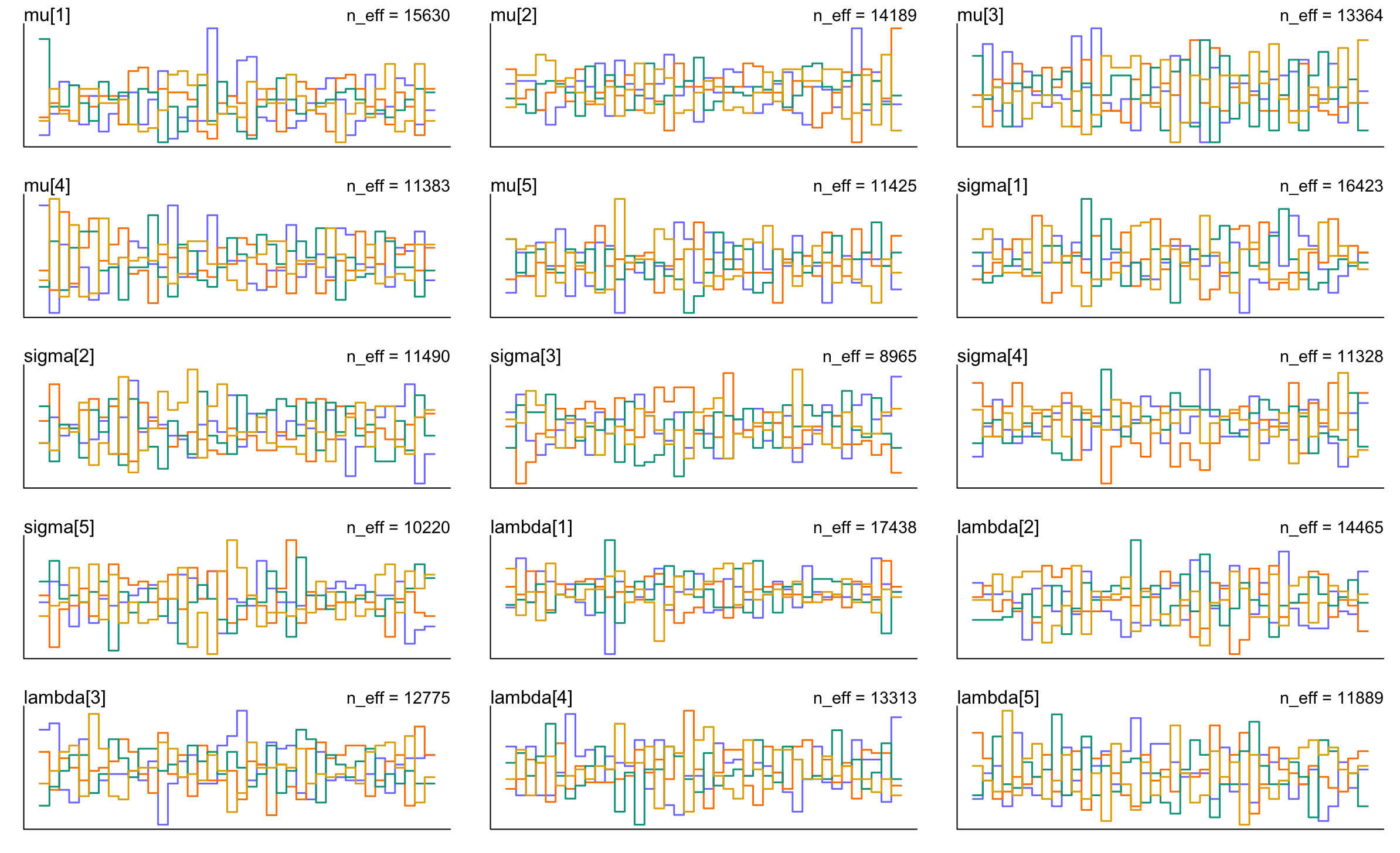
When I ran NCP#1 on my simulated dataset, and it did horribly (the traceplots look like a Jackson Polock, and only the \lambda_k's were properly recovered). I haven’t even bothered to run it on the real data.
- 375 divergent transitions after warmup
- 3625 transitions after warmup that exceeded the maximum treedepth
- Largest R-hat is 3.76 (run for more iterations may help)
- Bulk ESS is too low (run for more iterations may help)
- Tail ESS is too low (run for more iterations may help)
I thought that maybe the geometry was still too tricky, so I wrote and tried to run my fully-non-centered parameterization, but I clearly wrote it wrong, because it refuses to compile (I can’t figure out how to set x[j]=anything while I declare vector[nCall] x in the data section; and I also can’t figure out what I would write like x[j]~something in order to get x to follow a non-centered parameterization).
This is where I realized “wow, am I out of my depth, I need help.” If you have any thoughts about how to fix my models, Stan, or anything else, or if you have or any reading I should do to help clarify what Stan is doing with my code, I would be so grateful. Thank you in advance.