Seeking posterior predictive distributions for 727 parameters (lakes) that are destinations for seaplane pilots but where a portion of the flights originates from source lakes harboring aquatic invasive species. I am modeling this like trials using a hierarchical binomial model just like the rats tumor example to keep it simple. Have data for over 25000 flights but some of the lakes only receive a handfull of flights.
Model runs fine but:
max tree depth reached each time I increase, most recently to 15, but still same warning messages
cannot open pairs() plot as suggested Error in plot.new(): figure margins too large
half of the lakes have Rhat larger than 1.1
Some of the Rhat >1.1 lakes have chains that run parallel horizontally, not mixing
Increased iterations from 2000 to 10000 and most recently 20000 (took 4 days to run with multiple processors etc.) same warnings
bulk ESS too low
tail ESS too low
Used launch_shinystan but found no issues with divergence. So I am wondering given the very large number of parameters/predictive distributions whether the diagnostics are to be expected and as good/simple as we can get here. The distributions will inform detection efforts to survey lakes that show high median introduction rates (tumor successes) first the ones with low variance then the ones with higher variance.
Here is the model:
J <- nrow(data)
n <- data$flights
y <- data$eflights  # flights from invader source lakes
library(rstan)
rstan_options(auto_write = TRUE)
Sys.setenv(LOCAL_CPPFLAGS = '-march=native')
options(mc.cores = parallel::detectCores())
datafit3 <- stan(file="STAN/flights_model/flights_model.stan",data=c("J","y","n"), iter = 20000, chains = 4,control=list(adapt_delta=0.8, max_treedepth =15))
Stancode
// Following Carpenter et al. 2016 p. 16
data {
  int<lower=0> J; // number of lakes
  int<lower=0> y[J]; // number of flights from elodea-invaded sources into lake j
  int<lower=0> n[J]; // number of total flights into lake j (number of trials)
}
parameters {
  real<lower=0,upper=1> theta[J]; // chances of success
  real<lower=0,upper=1> lambda; // prior mean chance of success
  real<lower=0.1> kappa; // prior count
}
transformed parameters {
  real<lower=0> alpha; // prior success count
  real<lower=0> beta; // prior failure count
  alpha = lambda* kappa;   //alpha parameter for the prior
  beta =   (1 - lambda)* kappa;  //beta parameter for the prior
}
model {
  lambda ~ uniform(0,1); // hyperprior
  kappa ~ pareto(0.1,1.5); // hyperprior was uniform(0.1,5) for results as of 04/30/20 creating datafit1, pareto(0.1,1.5) creating datafit2, uniform(0,1) in Carpenter et al.
  theta ~ beta(alpha,beta); // prior for the probability p that lake j is invaded
  y ~ binomial(n,theta); // likelihood for flights

}
generated quantities {
  real<lower=0,upper=1> avg; // avg success
  int<lower=0,upper=1> above_avg[J]; // true if theta[j] > mean(theta), meaning the posterior prob. that a given destination is above-average in terms of the elodea introduction rate
  int<lower=1,upper=J> rnk[J]; // rank of j
  int<lower=0,upper=1> highest[J]; // true if j is highest rank
  avg = mean(theta);
    for (j in 1:J)
    above_avg[j] = (theta[j] > avg);
    for (j in 1:J) {
    rnk[j] = rank(theta,j) + 1;
    highest[j] = rnk[j] == 1;
  }
}
The automatic ESS messages will break (yielding a false warning) if you have any variables that are constant in the generated quantities, which might be happening with some of those int quantities. If the model doesn’t take too long to run, try running without any generated quantities to check if you still get ESS warnings.
When you say that you’re seeing rhat’s >1.1 for some lakes, do you mean for the theta for some lakes?
The pairs plot worked out, just by limiting the number of plots to be displayed.
The neff/N ratios are super small for most lakes. I am unfamiliar with reparameterization but would it perhaps help here? If so, how would the model need to be reparameterized? Thanks so much for your help.
Andrew, I switched the code following your example but the code file shows a warning on the line I inserted it in the generated quantities block (white x on round red background):
“No matches for: Available argument signatures for operator+: Expression is ill formed.”
Hi Mike, sorry for the very delayed response and thanks so much again for your help.
I get the same errors with a smaller dataset. But I wonder if the error messages are actually not a large validity concern. Note, when I increased iterations from 10,000 to 20,000 after warm up, I had considerable better convergence. With 20,000 I got 200 (28% of the 727 lakes) with Rhat ≤ 1.05 instead of 41 lakes with 10,000 iterations, 457 (63%) instead of 224 with Rhat ≤ 1.1, and 270 (37%) instead of 503 lakes with Rhat > 1.1.
Since there are so many thetas and the data is somewhat sparse for some of these lakes with only a few flights going in, I believe the model may be as good as it gets. Is there reason to throw out the model entirely? Or could we interpret the results by saying the 200 lakes with Rhat ≤ 1.05 are “trust worthy” results, the estimates for the 457 lakes are “more or less trustworthy” and the 270 remaining lakes with Rhat >1.1 are potentially problematic.
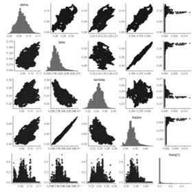
Btw, here is the pairsplot with just one of the 727 lakes. Are there any issues you see? I never interpreted these and don’t know what to look for. But, I noticed, with 10,000 iterations that some of the pairs had some bimodality that went away with 20,000 iterations.
Unfortunately I really don’t think it’s safe to ignore the Rhat warnings generally. They indicate that the different chains ended up exploring measurably different areas of the parameter space, so all computations on the resulting samples have no guarantee of accuracy. There’s even been talk of decreasing the Rhat value that triggers the warning to something even smaller like 1.01 to really ensure folks only trust samples from truly converged chains.
Maybe you need to step back and reconsider this model for the data. You should check out @betanalpha’s workflow case study and do those same steps yourself.
There are some visible “loops” indicating very slow mixing. Max tree depth warning also indicates very small step size and thus many many steps are needed before u-turn. The figure you attached is too small to see anything else (like axis labels). Can you post a bigger figure?
I don’t still see the problem, but this are rare type of example with very slow mixing.
To better see the geometry can you plot the pairs plot in the unconstrained space (where the sampling happens), that is for kappa plot log(kappa-0.1), for theta and lambda plot logit(theta) and logit(lambda)?
Not sure if this is correct to get the transformations you want pairs_plot2 <- mcmc_pairs(posterior_cp, np = np_cp, pars = c("alpha","beta","logit(lambda)","log(kappa,-0.1)","logit(theta[1])"), off_diag_args = list(size = 0.75))
How does the plot with that call look like? My current guess is that with the current priors you have way too much prior mass on very small theta values, which in logit space means that the tail is thick and it takes forever to explore that tail. We could see that better when looking the posterior in the unconstrained space and the way to fix it would be to use slightly more informative prior.
The pairs plots of theta[1] against the other parameters indicate that something in the model is being terribly identified. See https://betanalpha.github.io/assets/case_studies/identifiability.html for recommendations on how to access the unconstrained values as well as some explanation for why extremely degenerate models like this will appear to be multimodal for if the Markov chains aren’t long enough.
Does that give you an error? Unless you’ve created variables with those names, you need pars to be the actual parameter names and to then use the transformations argument to provide the functions. The way you currently have it it will look for a parameter named “logit(lambda)” rather than applying the logit transformation to “lambda”. Something like this should work:
pairs_plot2 <-
  mcmc_pairs(
    posterior_cp,
    np = np_cp,
    pars = c("alpha", "beta", "lambda", "kappa", "theta[1]"),
    transformations = list(
      "lambda" = "qlogis",  # or define a function called logit
      "kappa" = function(x) log(x - 0.1),
      "theta[1]" = "qlogis"
    ),
    off_diag_args = list(size = 0.75)
  )
Alternatively, you can do what @betanalpha suggested and just extract and plot the already unconstrained draws themselves.
The above code for the pairs_plot gave me an error, so I used @jonah’s suggestion specifying the transformation argument. The resulting pairs_plot is exactly the same. Hmm?
If I undersand correctly, following @betanalpha suggestion would mean looking at the diagnostic_file which unfortunately, I did not specify. The model ran for four days on 8 cores. Happy to rerun it though or just use fewer iterations.
If the model takes that long to run then it will be much faster to create the pairs scatter plots one by one, and imposing the unconstraining transformations, by hand.