Best linear fit through the initial part of data

Hello,

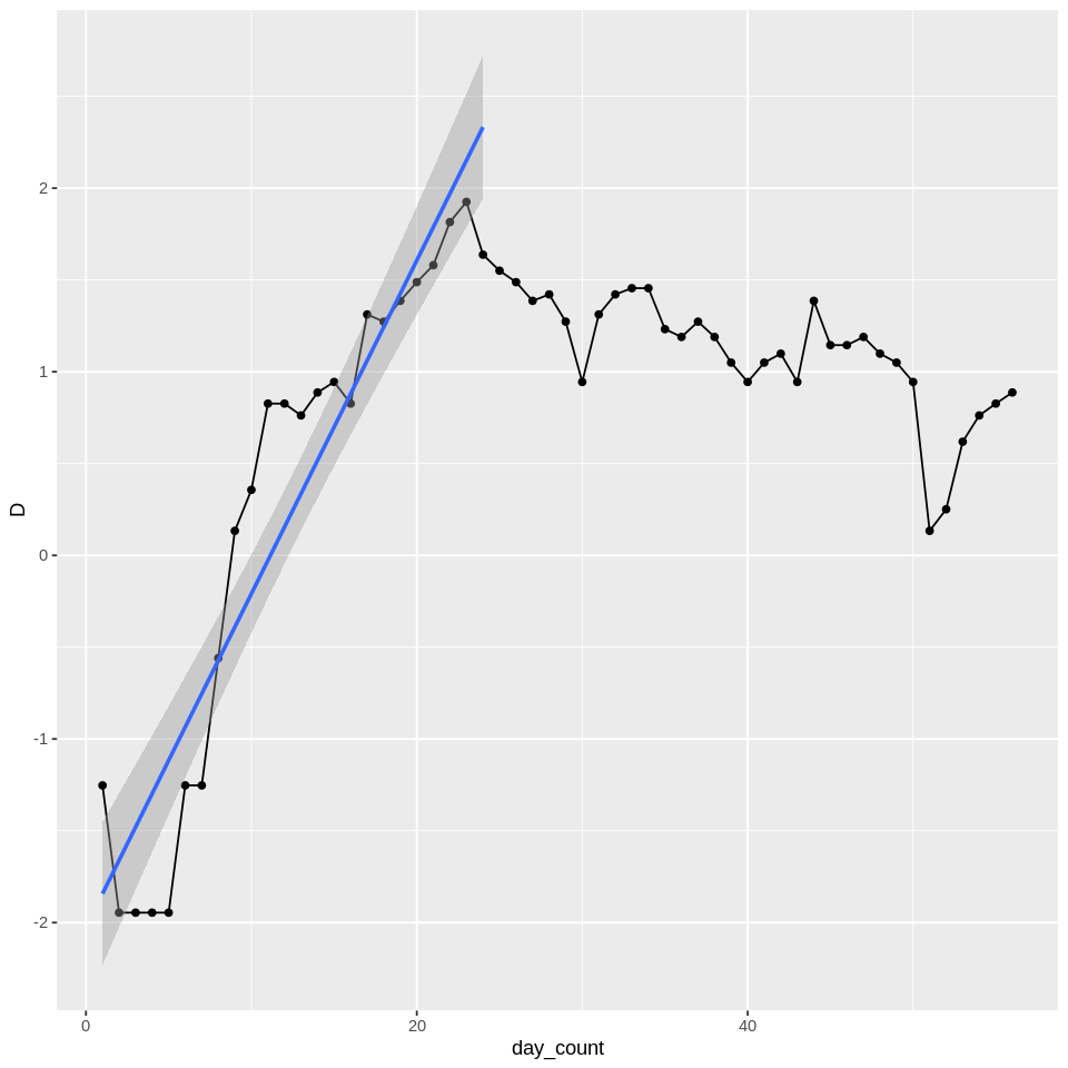
I am new to Stan and I am trying to fit a simple linear model to daily data D, but I want the fit to be only to the initial part of the data that fits the best. In R, I can do this by starting from the first observation and gradually including new observations until the fit worsens. I have included a plot for what I want the fit to look like. Is there a way to do a similar fit in Stan?

I followed the Change Point example in the manual here https://mc-stan.org/docs/2_21/stan-users-guide/change-point-section.html. That example marginalizes the change point, and finds a change point and fits two models: one to the early part of the data and one to the later part. I thought that I can also marginalize the change point and ignore the later part of the data by only computing the log_likelihood for the early part. So, I changed the inner loop to 1:s instead of 1:T so that the data likelihood is only computed up to the change point, but that didn’t work. I am not sure what I am doing wrong. Here is my R and Stan code based on the change point example.

Thanks!

test_stan|500x500

day_count <- c(1:56) 
D <- c(-1.252763,-1.9459101,-1.9459101,-1.9459101,-1.9459101,-1.252763,-1.252763,-0.5596158,0.1335314,0.3566749,0.8266786,0.8266786,0.7621401,0.8873032,0.9444616,0.8266786,1.3121864,1.2729657,1.3862944,1.4880771,1.5804504,1.81529,1.9252909,1.6376088,1.5505974,1.4880771,1.3862944,1.4213857,1.2729657,0.9444616,1.3121864,1.4213857,1.4552872,1.4552872,1.2321437,1.1895841,1.2729657,1.1895841,1.0498221,0.9444616,1.0498221,1.0986123,0.9444616,1.3862944,1.1451323,1.1451323,1.1895841,1.0986123,1.0498221,0.9444616,0.1335314,0.2513144,0.6190392,0.7621401,0.8266786,0.8873032)

test <- list(T = length(day_count), 
                     day_count = day_count,
                     D = D)

fit <- stan(file = 'best_fit.stan', data = test, chains = 1)

data {
  int<lower=1> T;
  vector[T] day_count;
  real D[T];
}
transformed data {
  real log_unif;
  log_unif = -log(T);
}
parameters {
  real<lower=0> sigma;
  real a0;
  real<lower=0> a1;
}
transformed parameters {
  vector[T] mu = a0 + a1 * day_count;
  vector[T] lp;
  lp = rep_vector(log_unif, T);
  for (s in 1:T)
    for (t in 1:s)
      lp[s] = lp[s] + normal_lpdf(D[t] | mu[t], sigma);
}
model {
  target += log_sum_exp(lp);
}

You need to leave both parts of the change point code in . Once it’s fitted then just use the first part. A change point can’t be determined without actually fitting the model after the changepoint.

Although I’m not sure you’ll get what you’re hoping for like this. Your graph could have 10 change points in it. If you fit just two, your lines could be arbitrarily polluted. In my limited experience, there’s no good way to determine how many change points a dataset has, and if you try and work with more than two change points you’ll quickly find that the model won’t identify because there’ll likely be multiple solutions which work just as well for anything non trivial.

Thank you emiruz for your response. I thought about using both parts to the change model and keeping the first part, but the problem like you said is that I have multiple trends and they are very different. So, it may be very difficult to get a change point model to work correctly. I was hoping that there may be another approach that could work better than a change point model. In R, I simply increase the window size from left to right, compute the R^2 and then go back and get the linear fit which had the best R^2. With a bit of tuning, that seemed to work relatively well. So, I considered passing the R^2 to Stan and work with that in Stan, but I it would be great if there is another way to get to a similar result directly in Stan.

I’m not sure sorry. You could try differencing your series and looking to see it that gives you something more to work with. Or you could look into sequential change point algorithms ( which are typically not Bayesian).

No worries emiruz. I figured out a solution that seems to be working so far. I am posting the code here for others in case someone may have a similar question or can think of a way to improve the code.

The answer was actually not that hard. I assigned a weight to each one of the days using a probit function. So, the earlier days are weighted higher and the later dates are weighted lower. The weights are determined by two parameters a center (day_count0) and a scaling factor f. Then, I simply apply the weight to the log likelihood and so far it seems to be working well.!

download (1)|500x500

data {
  int<lower=1> T;
  vector[T] day_count;
  real D[T];
}
parameters {
  real<lower=0> sigma;
  real a0;
  real<lower=0> a1;
  real<lower=day_count[5], upper=day_count[T]> day_count0; //inflection point for the probit weights
  real<lower=1, upper=sd(day_count)> f; // logistic scaling to determine cutoff
}
transformed parameters {
  vector[T] mu = a0 + a1 * day_count;
  vector[T] exp_probit = exp((day_count0 - day_count) / f);  
  vector[T] weights = exp_probit ./ (1 + exp_probit); 
}
model {
  for(i in 1:T){ 
     target += normal_lpdf(D[i] | mu[i], sigma) * weights[i]; 
  }
}