Issues with poisson changepoint model

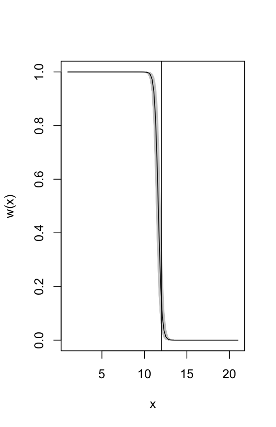
Hi any and all Stan aficionados – I am having some trouble getting the following Poisson change point Stan model to run, the pairs plot seems to suggest that the slope and intercept variables within a change point are perfectly collinear. I am quite a novice for these issues so I was hoping I could defer to someone with more expertise in how to tackle this problem.

Stan code and simulated code to recreate my issue can be found below

data {
  // Define variables in data
  // Number of observations (an integer)
  int<lower=0> N;
  real x[N];
  // Count outcome
  int<lower=0> y[N];
}

parameters {
  real a1;
  real a2;
  real b1;
  real b2;
  real<lower=0> fixedkp;
}

transformed parameters  {
  //
  real lp[N];

  for (j in 1:N) {
    if (x[j] < fixedkp) 
      lp[j] <- a1 + b1*x[j];
    else  
      lp[j] <- a2 + b2*x[j];  
  }

}

model {
  // Prior part of Bayesian inference
  // Flat prior for mu (no need to specify if non-informative)
  a1 ~ normal(0,3);
  a2 ~ normal(0,3);
  b1 ~ normal(0,3);
  b2 ~ normal(0,3);
  fixedkp ~ uniform(1,30);

  // Likelihood part of Bayesian inference
  y ~ poisson_log(lp);
}

n1 <- 1000
n2 <- 1000
a1 <- 4
b1 <- -.2
a2 <- .5
b2 <- .0044
x1 <- sample(1:11, n1, replace=TRUE)
mu <- exp(a1 + b1 * x1 + rnorm(n1,.2,.3))
y1 <- rpois(n=n1, lambda=mu)
x2 <- sample(12:21, n2, replace=TRUE)
mu <- exp(a2 + b2 * x2 + rnorm(n2, .2,.3))
y2 <- rpois(n=n2, lambda=mu)
## Now make the data frame
out.dat = data.frame(y = c(y1, y2), x = c(x1, x2))
stan.data = list(
    N = nrow(out.dat),
    x = out.dat$x,
    y = out.dat$y
)
plot(out.dat$x, out.dat$y)
stanmonitor <- c("a1","a2","b1","b2","fixedkp")
mod <- stan(file="/home/arosen/Documents/pinesRep/scripts/stan_models/singleBasePoisCP.stan", 
    data = stan.data, cores=4,
    pars = stanmonitor, 
    iter=1000, warmup = 500, control = list(adapt_delta = 0.9, max_treedepth = 15))

There are a few syntax errors in your provided Stan code. The following complies and runs with cmdstanr 0.8.1:

data {
  // Define variables in data
  // Number of observations (an integer)
  int<lower=0> N;
  vector[N] x;
  // Count outcome
  array[N] int<lower=0> y;
}

parameters {
  real a1;
  real a2;
  real b1;
  real b2;
  real<lower=0,upper=21> fixedkp;
}

transformed parameters  {
  //
  vector[N] lp;

  for (j in 1:N) {
    if (x[j] < fixedkp) 
      lp[j] = a1 + b1*x[j];
    else  
      lp[j] = a2 + b2*x[j];  
  }

}

Second, the normal noise added in constructing the mu term, e.g.:

mu <- exp(a1 + b1 * x1 + rnorm(n1,.2,.3))

does not appear in the Stan model, which will probably cause issues with recovering the true parameter values.

Finally, the model as currently specified is probably not identifiable under the uniform prior on the changepoint location. I was able to get things to work with a normal(10,3) prior on the changepoint – you may want to think about if your problem lends itself to at least a weakly informative prior. Alternatively, you may also wish to investigate if the mean function needs to be discontinuous at the changepoint. If not you might have better efficiency working with splines.

Hi @js592 thanks for looking over my code – I couldn’t exactly find where you changed my Stan code, could you provide some hints?

My concern wasn’t getting with the Stan code compiled, although your tips did improve speed of the model slightly, the bigger issue was how my within change point slope parameter estimation distribution are highly correlated, if you look at the pairs plot of the output there appears to be strong correlation between the A1 & B1 parameters.

Is this the model identification issue you’re alluding to?

Sure. These lp[j] <- a1 + b1*x[j] lines originally used <- instead of =, I switched the real foo[N] notation to vector[N] foo, and the int foo[N] to array[N] int foo. You might be using a version of Rstan that doesn’t incorporate the updated array syntax, so it might not necessarily be that big of an issue.

With regards to identifiability it was more a comment about how if you are modeling knots or changepoints (as opposed to fixing them a priori, which is probably more common) you probably want at least a weakly informative prior – otherwise, the model can end up being flexible enough that many different choices of knot/changepoint location can fit the data well.

However, I suspect most of the issues you may have with this model arise because of how the discontiunity is formulated. I have not explored this concept in depth myself but I believe HMC will struggle becuase the likelihood itself becomes discontinuous (e.g. Modeling Cutpoint for Noisy Covariate - #5 by icostley or https://statmodeling.stat.columbia.edu/2017/05/19/continuous-hinge-function-bayesian-modeling/
Like I said earlier, you may want to think about the physics of what you are trying to model and decide if the true behavior really has an instantaneous jump or actually has a very rapid smooth transition. The latter I think should be much more ammendable to HMC.

1 Like

I wanted to add a bit more to my response that I hope will clarify some of the points I raised above. One way to model a smooth transitions between two data regimes looks like:
\log \mu(x) = w(x)f_1(x)+(1-w(x))f_2(x)
where f_1(x) = a_1+b_1x, f_2(x) = a_2 + b_2x, and w(x) is some function that lives between [0,1]. Because our domain expertise informs us that there should only be one changepoint with a clear transition a natural choice for w(x) might be the inverse logit:
w(x) = \frac{1}{1+exp(-(\alpha + \beta x)}
This has the properties of saturating at 0 and 1 which will allow for clear separation between the two regimes. The steepness (how sharp the transition is) is given by \beta and the midpoint (where w(x) = 0.5) is -\alpha/\beta. The stan code below estimates a model where we a priori fix \beta = -5 and pass it as data (one could also choose to estimate it and impose an informative prior to the same effect).

data {
  // Define variables in data
  // Number of observations (an integer)
  int<lower=0> N;
  vector[N] x;
  // Count outcome
  array[N] int<lower=0> y;
  real beta; //fixed gain of logistic changepoint
}

parameters {
  real a1;
  real a2;
  real b1;
  real b2;
  real<lower=-1*beta, upper =-21*beta>  alpha;

}

transformed parameters  {
  vector[N] w = inv_logit(alpha + beta*x);
}

model {
  // Prior part of Bayesian inference
  a1 ~ normal(0,3);
  a2 ~ normal(0,3);
  b1 ~ normal(0,3);
  b2 ~ normal(0,3);
  //implicitly, there is a uniform(1,21) prior on the changepoint (middle of logistic weighting curve)

  vector[N] lp;

  lp = w.*(a1 + b1*x) + (1-w).*(a2 + b2*x);

  // Likelihood part of Bayesian inference
  y ~ poisson_log(lp);
}

For me, this runs quite fast and has no divergent transitions or treedepth warnings even without tinkering with the adapt_delta setting. The parameter recovery is good:


As is the changepoint estimation (here I show the posterior mean and 500 draws):

One thing to note about that uniform prior, however, is very rarely with the random initalization a chain can get stuck on the boundary value of the changepoint. This I think corresponds to essentially no changepoint and may happen because the data is also reasonably modeled by a single continuous linear function for the Poisson mean. I was able to solve this with a diffuse normal prior on \alpha centered in the middle of the interval of x values (e.g. something like N(55,5)).

For the collinearity, it still appears somewhat:


However, I suspect that this may be more of a result of the assumed data generating process instead of an inherent degeneracy. It may be worth exploring different assumed values of the slopes, intercepts, and changepoint and seeing if the problem persists.

PS: With the simulated values for x only taking integer values you might run into some issues where the data cannot inform where exactly in the interval [11,12] the change occurs.

4 Likes

absolutely gorgeous! I very much appreciate your insight!

Hi @js592

I am trying to extend this model into a 2 chnage point model, I thought I could do this using your same inv_logit formulation but now do it as an ordered inv_logit. So my model weights now become:

  vector[N] w1;
  vector[N] w2;
  vector[N] w3;
  w1 = inv_logit(beta + alpha[1]*x);
  w2 = inv_logit(beta + alpha[2]*x) - inv_logit(beta + alpha[1]*x);
  w3 = 1 - inv_logit(beta + alpha[2]*x);

and my model now becomes:

    lp[j] = w1[j]*(a1+b1*x[j])+
      w2[j]*(a2+b2*x[j])+
      w3[j]*(a3+b3*x[j]);

Where a’s represent intercept terms, b’s represent slope terms. This model is returning nonsense, though, I can’t seem to be able to estimate anything meaningful using this formulation. Would you happen to have ideas for how you would approach this problem?

I’m a bit busy at the moment so I can’t dive too deep into this. My suggestion would be if you want to model multiple switches between two regimes you could stick with original formula but instead of having the a linear function (alpha + beta*x) switch to something that can “wiggle” up and down a bit more. Maybe a linear spline with one or two knots or even a Gaussian process. But I’d expect a lot more identifiability issues. On the other hand, if you want to model multiple regimes I would look into a hidden markov model or something similar.

1 Like

got it, thanks @js592