Balancing loo performance and Prior sensitivity analysis

Hi,

While building models and trying out different priors, I noticed that using a prior that seemed more sensible based on my sensitivity analysis decreased my loo performance. The old prior, the one before the sensitivity analysis, also seems to sample slightly better.

Would it be correct to go with the old priors based on those facts, even though the sensitivity analysis made the new priors seem like a better choice?
I put the brms code for both models below.

old.priors = brm(
  formula = EXAM ~ 1 + Weighting + LOC + (1|Project),
  data = ls.df,
  family=Beta(),
  prior = c(
    prior(normal(0,10), class=Intercept),
    prior(normal(0,0.5), class=b),
    prior(cauchy(0,0.5), class=sd),
    prior(gamma(0.1, 0.1), class=phi)
  )
)

new.priors = brm(
  formula = EXAM ~ 1 + Weighting + LOC + (1|Project),
  data = ls.df,
  family=Beta(),
  prior = c(
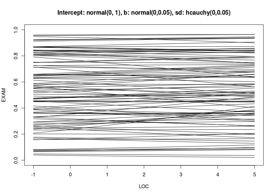
    prior(normal(0,1), class=Intercept),
    prior(normal(0,0.05), class=b),
    prior(cauchy(0,0.05), class=sd),
    prior(gamma(0.1, 0.1), class=phi)
  )
)

One guess is that my prior sensitivity analysis is not correct. I tried following McElreath’s book but I didn’t find examples for how to do it for varying intercepts so I tried to come up with something myself.
If I understand it right, I might have to make multiple plots (or multidimensional plots, one for each parameter) so maybe that is my error?

sensitivity<- function(intercept, parameters, var_intercepts) {
  N = 100
  
  b_intercept = rnorm(N, 0, intercept)
  b_weighting = rnorm(N, 0, parameters)
  b_loc = rnorm(N, 0, parameters)
  m_project = rhcauchy(N, var_intercepts)
  
  b_project = rep(0, N)
  for (i in 1:N) {
    b_project[i] = rnorm(1, m_project, intercept)
  }
  
  for (w in 0:1){
    plot(NULL, xlim = c(-1, 5), ylim = c(0, 1))
    for (i in 1:N) {
      curve(exp(b_intercept[i] + b_weighting[i] * w + b_loc[i] * x + b_project[i]) / (
        1 + exp(b_intercept[i] + b_weighting[i] * w + b_loc[i] * x + b_project[i])
      ) ,
      add = TRUE)
    }  
  }
  
}

sensitivity(10, 10, 10)
...

Can you show the loo output for both cases so I can comment whether the difference is practically significant?

1 Like
           elpd_diff se_diff
old.priors  0.0       0.0   
new.priors -4.3       1.4 

As I understand it, you want the elpd_diff to be at least twice the se_diff, which would mean a significant difference here.

I also noticed, that both of them don’t sample too well. The n_eff for the intercept is just below 10% of post wamup samples for both of them, which is not enough I think. Rhat is 1.01 for both intercepts as well. So maybe comparing them is useless if they don’t sample properly anyway?
I tried a wider gamma prior gamma(1,1) for both of them and they both reach the 10% post warmup samples now and the loo_compare gives this:

           elpd_diff se_diff
old.priors  0.0       0.0   
new.priors -6.2       1.1  

Which is even more significant from what I understand.

The problem is that the current se_diff estimate is underestimate and it would be safer to have at least four times the se_diff (we’re in progress of writing more about this)

That’s right. 10% is not bad if total number of iterations is large enough. Don’t look at the percentage look at the n_eff.

Can you also show loo output for each model as it contains diagnostics for loo computation.

> loo(old.priors)

Computed from 4000 by 378 log-likelihood matrix

         Estimate   SE
elpd_loo    795.3 14.5
p_loo        18.7  1.4
looic     -1590.7 28.9
------
Monte Carlo SE of elpd_loo is 0.1.

All Pareto k estimates are good (k < 0.5).
See help('pareto-k-diagnostic') for details.
> loo(new.priors)

Computed from 4000 by 378 log-likelihood matrix

         Estimate   SE
elpd_loo    791.1 13.9
p_loo        18.5  1.3
looic     -1582.2 27.8
------
Monte Carlo SE of elpd_loo is 0.1.

All Pareto k estimates are good (k < 0.5).
See help('pareto-k-diagnostic') for details.

I found n_eff/N > 0.001 on the stan developer best practices guide so maybe those n_eff are fine after all.

loo diagnostics look good. Your new priors are likely to be too tight.

What did you do for sensitivity analysis?

Ah, we should update that to follow the new recommendations in [1903.08008] Rank-normalization, folding, and localization: An improved $\widehat{R}$ for assessing convergence of MCMC

I used the sensitivity function from my first post and played around with the numbers to get something that looked like a pretty even distribution over all the space.
I wasn’t really sure how to do that right as I haven’t seen examples using a logit link or varying intercepts so I guess there is a good chance that its not correct?

Here is the code again:

library(extraDistr)
sensitivity<- function(intercept, parameters, var_intercepts) {
  N = 100
  
  b_intercept = rnorm(N, 0, intercept)
  b_weighting = rnorm(N, 0, parameters)
  b_loc = rnorm(N, 0, parameters)
  m_project = rhcauchy(N, var_intercepts)
  
  b_project = rep(0, N)
  for (i in 1:N) {
    b_project[i] = rnorm(1, m_project, intercept)
  }
  
  for (w in 0:1){
    plot(NULL, xlim = c(-1, 5), ylim = c(0, 1))
    for (i in 1:N) {
      curve(exp(b_intercept[i] + b_weighting[i] * w + b_loc[i] * x + b_project[i]) / (
        1 + exp(b_intercept[i] + b_weighting[i] * w + b_loc[i] * x + b_project[i])
      ) ,
      add = TRUE)
    }  
  }
  
}

sensitivity(10, 10, 10)
...

Can you post some figures with explanations how to interpret sensitivity from those?

I started with this prior as a starting point:


My interpretation of this was, that most of the curves were too steep. For most of the parameter space a unit chance in LOO would have no impact on the output. At the same time a small difference close to the tipping point would completely flip the output around. This felt like putting too much weight on big changes.

Next step:


This is what I used as the “old prior”.
This I interpreted as having too much weight on the extremes as only a few curves had moved between 0 and 1 over the parameter space.

Next step:


This is what I used as the “new prior”.
I now realize, that I had a typo in my model which is why the b and sd priors are so narrow.
However plotting the priors like this now makes me realize, that they seem so flat, that for almost none of the curves a change in LOC does anything to the output.
This seems too narrow from the picture.

Next step:


This is what I wanted to use as the new prior.
Here it seems like most of the curves are able to move between 0 and 1 and there is not too much weight on any extremes besides maybe a little bit too much for high LOC values. However it looks a lot more evenly distributed than the ones before.

Comparing the two models from the first post with a model using the priors from the last picture results in this (m1.3 is the new model):

           elpd_diff se_diff
old.priors  0.0       0.0   
m1.3       -0.2       0.1   
new.priors -4.3       1.4  

It looks like the old priors and m1.3 have very similar loo performance but m1.3 samples a little bit better than other two models. Although n_eff of m1.3 is still only 383, so less than 10% of post warmup samples and rhat is 1.01 (which is ok I think).
So my confusion probably stems from me making a typo when adding the priors that looked fine in the analysis into the model. Being too narrow then hurt the performance.

1 Like

Excellent figures. It seems the mystery is now solved?

1 Like

Thank you. And yes, I think it comes down to a typo in the end :)