Aggregated model for mixture of Exponential distributions

Hey everyone!
I’m working on a time-to-event model. Waiting times come from a mixture of two exponential distributions, with a low- (e.g., 20 minutes) and a high (e.g., 5000 minutes) averages. After a certain waiting time (e.g., 40 minutes), observations are censored.

Small R simulation:

# Number of observations
N <- 100

# Average holding times 
theta <- sample(c(20, 5e3), N, replace = TRUE, prob = c(0.3, 0.7))

# True holding times
X_true <- rexp(N, 1 / theta)

# data input for Stan
d <- list()
d$N <- N

# Was the holding time censored?
d$C <- ifelse(X_true > 40, 1, 0)

# Observed holding time
d$X <- ifelse(d$C == 1, 40, X_true)

# Total time spent waiting
d$exposure <- sum(d$X)

# Number of observed events
d$count <- sum(df$C == 0)

I want to recover the means of the two exponential distributions. To do so, I wrote a first Stan model:

  data{
  int<lower = 0> N;                     // Number of observations
  array[N] int<lower = 0, upper = 1> C; // Censoring level
  vector[N] X;                          // Waiting times
}

parameters {
  real<lower = 0> theta_1;              // Low mean
  real<lower = theta_1> theta_2;        // High mean
  real<lower = 0, upper = 1> omega;     // Mixture weight
}

model {
  // Priors
  target += normal_lpdf(theta_1 | 30, 10);
  target += normal_lpdf(theta_2 | 3e3, 3e3);
  target += beta_lpdf(omega | 2, 2);

  // Likelihood
  for (n in 1:N) {
    // Non-censored cases
    if(C[n] == 0){
    target += log_mix(omega,
                      exponential_lpdf(X[n] | 1.0 / theta_1),
                      exponential_lpdf(X[n] | 1.0 / theta_2));
    }
    // Censored cases
    if (C[n] == 1){
    target += log_mix(omega,
                      exponential_lccdf(X[n] | 1.0 / theta_1),
                      exponential_lccdf(X[n] | 1.0 / theta_2));
    } // if
  } // n
} // model block

It seems to work fine. However, I’d like—if possible—to code a more computationally efficient version of the model by aggregating the data. I know that a Poisson process can be described by either exponentially-distributed waiting times:

X_{j} \sim \text{Exponential}(1 / \theta),

Or by a Poisson distribution:

\sum_j \mathbb{I}(C_{j} = 0) \sim \text{Poisson}(\sum_{j}X_{j} / \theta)

However, I wonder whether the aggregated/Poisson strategy can also be applied to the mixture described above. My naive attempt was to try the following:

data{
  int<lower = 0> count;                 // Number of non-censored observations
  real exposure;                        // Sum of all holding times
}

parameters {
  real<lower = 0> theta_1;              // Low mean
  real<lower = theta_1> theta_2;        // High mean
  real<lower = 0, upper = 1> omega;     // Mixture weight
}

model {
  // Priors
  target += normal_lpdf(theta_1 | 30, 10);
  target += normal_lpdf(theta_2 | 3e3, 3e3);
  target += beta_lpdf(omega | 2, 2);

  // Likelihood
    target += log_mix(omega,
                      poisson_lpmf(count | exposure / theta_1),
                      poisson_lpmf(count | exposure / theta_2));

}

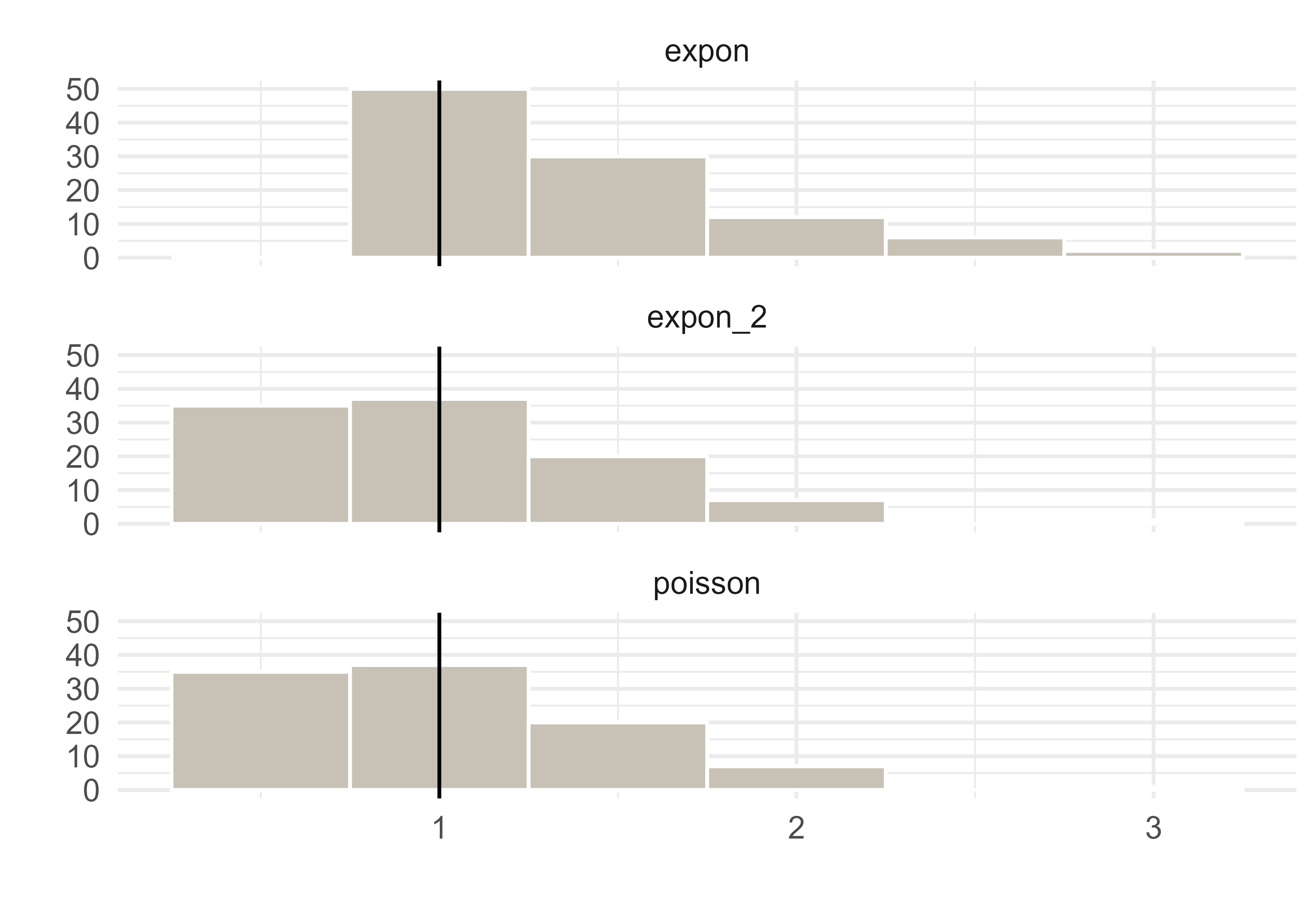
However, it doesn’t seem to recover the true means. Is there a way of making this work?
Please let me know if anything is unclear. Thanks for your time!
Ben

Hi, @BenKawam, and welcome to the Stan forums.

This is problematic:

  target += normal_lpdf(theta_1 | 30, 10);
  target += normal_lpdf(theta_2 | 3e3, 3e3);

You’ve put variables on huge scales, whereas Stan assumes for initialization that everything’s unit scale. So it’s going to initialize theta_1 and theta_2 in the (exp(-2), exp(2)) range, which is grossly misspecified for the priors.

I would suggest flipping this around and parameterizing this way for ordered rates:

real<lower=0, upper=1> theta_1;
real<lower=theta_1, upper=1> theta_2;

Now uniform priors are proper, but you could add beta priors if you wanted on top of that. Then the mixture would have exposure * theta_1 and exposure * theta_2 and the high/low direction flip.

We know that if we have a bunch of Poisson distributed variables that their sum is Poisson with the rate equal to the sum of the individual rates, i.e., y_n \sim \text{Poisson}(\lambda_n) implies \sum_n y_n \sim \text{Poisson}(\sum_n \lambda_n). But that doesn’t make the latter a good way to do estimation! It loses all the information linking the individual y_n to the individual \lambda_n. I didn’t understand your notation for the Poisson. It sounds like you’re instead talking about the relation between exponentials and Poissons, but you’re going to run into the same problem with reductions. Copying from the Wikipedia page on the Poisson:

If for every t > 0 the number of arrivals in the time interval [0, t] follows the Poisson distribution with mean λt, then the sequence of inter-arrival times are independent and identically distributed exponential random variables having mean 1/λ.

I don’t understand how the summation of indicator functions you wrote down relates to this. I’m guessing it’s still going to lose information compared to the exponential formulation.

Hi Bob, thanks so much for your help.

Your comments and suggestions for the parameters’ scale make sense to me! I’m still a bit confused about the Exponential/Poisson part, though. I’ll try to explain what I had in mind in more details.

As far as I understand—and I’m still very much new to this, so it might be nonsense—a Poisson process with rate 1 / \theta can be described either in terms of the exponentially-distributed waiting/interarrival times X^{\text{true}} between events:

X_{j}^{\text{true}} \sim \text{Exponential}(1 / \theta),

Or instead, in terms of number of events Y that happen over a certain period of exposure D:

Y \sim \text{Poisson}(D / \theta).

I simulate a small system with exponentially-distributed waiting times X_{j}^{\text{true}} where j \in \{1, ..., N\}.
These observations are censored if the waiting time is larger than a certain threshold.
I call X_{j} the observed (possibly censored) waiting times.

R code:

d <- list()
d$N <- 100

# True waiting times
d$X_true <- rexp(d$N, 1)

# Is the waiting time censored?
d$C <- ifelse(d$X_true > 1.5, 1, 0)

# Observed waiting time
d$X <- ifelse(d$C == 1, 1.5, d$X_true)

To recover \theta from X_{j}, we can model the non-censored observations using an Exponential-PDF, and the censored ones using an exponential-CCDF.

data{
  int<lower = 0> N;
  array[N] int<lower = 0, upper = 1> C;
  vector<lower = 0>[N] X;
}

parameters {
  real<lower = 0> theta;
}

model {
  target += exponential_lpdf(theta | 1);
  
  for (n in 1:N) {
    if(C[n] == 0){
      target += exponential_lpdf(X[n] | 1 / theta);
    }
    if(C[n] == 1){
      target += exponential_lccdf(X[n] | 1 / theta);
    } 
  }
}

An alternative (and perhaps weird) modelling strategy would be to have a Poisson outcome for each observation j. That is, we could model the number of events that have happened (0 or 1) for a given observation j, with the observed waiting time X_{j} as exposure time. I use an indicator variable here, \mathbb{I}(C_{j} = 0), taking a value of 1 if the waiting time is non-censored, and 0 otherwise.

\mathbb{I}(C_{j} = 0) \sim \text{Poisson}(X_{j} / \theta).

Now, indeed we can sum those events and rates because of the additivity of the Poisson process:

\sum_{j} \mathbb{I}(C_{j} = 0) \sim \text{Poisson}(\sum_{j} X_{j} / \theta).

Leading to the expression in my initial post. If I aggregate the simulated data in R:

d$count_non_censored_events <- sum(d$C == 0)
d$exposure <- sum(d$X)

And then run the following Stan model for the aggregated data:

data{
  int<lower = 0> count_non_censored_events;
  real<lower = 0> exposure;
}

parameters {
  real<lower = 0> theta;
}

model {
  target += exponential_lpdf(theta | 1);
  target += poisson_lpmf(count_non_censored_events | exposure / theta);
}

I can recover the rate \theta, too. The posterior distribution looks basically identical to the one of the first Stan model.

Is the above making any sense at all? Is it kosher? If it is, then my question was whether I could use the same kind of aggregation strategy when the observed waiting times come from a mixture of exponential distributions.

Finally, it might help if I add a word about the context, too: I want to do this because in my study system, I have hundreds of thousands of waiting times across less than a thousand units, and I only care about unit-level predictors, not about observation-level ones. I thus wanted to aggregate the observations within units to speed up computation.

What is the actual data you have? Is it data on waiting times or data on number of events over a certain period of exposure? If you have a lot of data it shouldn’t matter much, but if you don’t have much, then the exponential should be better.

Here’s a simple test that illustrates (ChatGPT (o3-mini-high) generated, then refactored to simplify).

expon.stan

data {
  int<lower=0> N;
  vector<lower=0>[N] w;
}
parameters {
  real<lower=0> lambda;
}
model {
  lambda ~ exponential(1);
  w ~ exponential(lambda);
}

poisson.stan

data {
real<lower=0> D;
int<lower=0> N;
}
parameters {
real<lower=0> lambda;
}
model {
lambda ~ exponential(1);
N ~ poisson(lambda * D);
}

pois-exp.py

import numpy as np
import cmdstanpy as csp
import logging
csp.utils.get_logger().setLevel(logging.ERROR)  # remove boilerplate & warnings

def simulate_poisson_process(D, rate=1.0):
    waiting_times = []
    cumulative = 0.0
    while True:
        wt = np.random.exponential(scale=1.0 / rate)
        if cumulative + wt > D:
            break
        waiting_times.append(wt)
        cumulative += wt
    return np.array(waiting_times)

def fit(stan_file, data):
    print(f"PROGRAM: {stan_file=}")
    model = csp.CmdStanModel(stan_file=stan_file)
    fit = model.sample(data = data, iter_sampling=50_000,
                           show_progress=False, show_console=False)
    print(fit.summary())
                           
for D in [1, 2, 4, 8, 16, 32]:
    print(f"{D=}")
    waiting_times = simulate_poisson_process(D, rate=1.0)
    N = len(waiting_times)
    data = {'D': D, 'N': N, 'w': waiting_times}
    fit("poisson.stan", data)
    fit("expon.stan", data)

You can see that the posteriors are not identical and are in fact way off for small total times D. As the number of waiting times increases, the estimates converge to the same posterior mean and standard deviation. This is using a lot of draws to get tight MCMC standard errors.

temp2$ python3 pois-exp.py

D=1
PROGRAM: stan_file='poisson.stan'
            Mean      MCSE    StdDev
lambda  0.500985  0.001909  0.504274

PROGRAM: stan_file='expon.stan'
           Mean      MCSE    StdDev
lambda  1.00104  0.003681  0.993824

D=2
PROGRAM: stan_file='poisson.stan'
           Mean      MCSE    StdDev 
lambda  1.00224  0.002254  0.579754

PROGRAM: stan_file='expon.stan'
           Mean      MCSE    StdDev
lambda  1.35185  0.003048  0.779444

D=4
PROGRAM: stan_file='poisson.stan'
            Mean      MCSE    StdDev 
lambda  0.799538  0.001422  0.399252

PROGRAM: stan_file='expon.stan'
           Mean      MCSE    StdDev       
lambda  2.02892  0.003902  1.018420 

D=8
PROGRAM: stan_file='poisson.stan'
           Mean      MCSE    StdDev       
lambda  0.88826  0.001125  0.313457 

PROGRAM: stan_file='expon.stan'
            Mean      MCSE    StdDev        
lambda  0.957637  0.001266  0.338883

D=16
PROGRAM: stan_file='poisson.stan'
            Mean     MCSE    StdDev     
lambda   0.70551  0.00073  0.203935

PROGRAM: stan_file='expon.stan'
            Mean      MCSE    StdDev      
lambda   0.75923  0.000809  0.218993

D=32
PROGRAM: stan_file='poisson.stan'
             Mean      MCSE    StdDev       
lambda    1.30372  0.000731  0.197708

PROGRAM: stan_file='expon.stan'
            Mean      MCSE    StdDev     
lambda   1.31289  0.000766  0.200372 

The mixture of two Poisson distributions isn’t Poisson any more—for example, it can be multimodal.

Now you could probably represent each mixture component this way, but in mixtures you have to be sure to include the normalizing constants.

Thanks again for your time and kind help, Bob!

“What is the actual data you have?”

I have the waiting times directly. I work with animal behaviour data. We record the behavioural events that an individual performs over a fixed amount of time (analogous to D in your simulations). From those, I deduce behavioural states, which I model using a kind of Continuous-Time Markov Chain where durations in behavioural states are exponentially-distributed, conditional on a set of variables.


I’ve never used Python, so my understanding of your code is rather approximate. I asked an R translation from Chat-GPT, who gave me this.

simulate_poisson_process <- function(D, rate = 1.0) {
  waiting_times <- numeric()
  cumulative <- 0.0
  while (TRUE) {
    wt <- rexp(1, rate = rate)
    if (cumulative + wt > D) break
    waiting_times <- c(waiting_times, wt)
    cumulative <- cumulative + wt
  }
  return(waiting_times)
}

The function generates a sequence of exponentially distributed waiting times, within a given period D, right? If so, then it makes sense to me that your two Stan models perform differently, because the last waiting time in your simulations, which is always censored, contributes to the likelihood only in poisson.stan, but not in expon.stan where only the non-censored waiting times are included. For this reason, I would actually expect poisson.stan to perform a bit better on average.

I quickly tried by running 100 iterations of the simulation for D = 1 (where we expect a larger difference between models):

D <- 1
n_iter <- 100
data <- list()
for(i in 1:n_iter){
  data[[i]] <- list()
  wt <- simulate_poisson_process(D)
  data[[i]]$w <- wt
  data[[i]]$N <- length(wt)
  data[[i]]$D <- D
  
  # New variables for expon_2.stan
  last_wt <- D - sum(wt)
  data[[i]]$new_w <- c(wt, last_wt)
  data[[i]]$c <- c(rep(0, length(wt)), 1)
}

I compare your Stan models with a third one that also includes the censored observations:

expon_2.stan

data {
  int<lower=0> N;
  vector<lower=0>[N+1] new_w;
  array[N+1] int<lower = 0, upper = 1> c;
}
parameters {
  real<lower=0> lambda;
}
model {
  lambda ~ exponential(1);
  for(i in 1:(N+1)){
    if(c[i] == 0) {
      target += exponential_lpdf(new_w[i] | lambda);
    } 
    if (c[i] == 1) {
      target += exponential_lccdf(new_w[i] | lambda);
    }
  }
}

I fit the 100 \times 3 models and plot the distribution of posterior means for \lambda.

# Packages
library(cmdstanr)
library(tidybayes)
library(tidyverse)

# Compile Stan models
models <- list(
  poisson = cmdstan_model("poisson.stan"),
  expon = cmdstan_model("expon.stan"),
  expon_2 = cmdstan_model("expon_2.stan")
)

posteriors <- list()
for (i in 1:n_iter) {
    for (m in 1:3) {
      posteriors[[paste0(m, "_", i)]] <- models[[m]]$sample(
        data = data[[i]],
        iter_warmup = 1e3,
        iter_sampling = 1e3,
        chains = 4,
        parallel_chains = 4
      )
      # Extract draws
      posteriors[[paste0(m, "_", i)]] <-
        tidy_draws(posteriors[[paste0(m, "_", i)]]) %>%
        mutate(iter = i,
               model = names(models)[m])
    } # m
} # i

# Plot
posteriors %>%
  bind_rows() %>%
  group_by(model, iter) %>%
  summarise(mean = mean(lambda)) %>%
  ggplot(aes(x = mean)) +
  geom_histogram(binwidth = 0.4, col = "white", fill = "#c7c2b5") +
  facet_wrap(~ model, nrow = 3) +
  geom_vline(xintercept = 1) +
  labs(x = "", y = "") +
  theme_minimal()

Here, expon.stan seems to overestimates \lambdai.e., it underestimates the distribution’s mean. I would guess this is partly because the large exponential draws are not included in the data set for expon.stan as they are larger than D. On the plot, we also see that the distribution of poisson.stan and expon_2.stan are close to identical. Please let me know if there is anything wrong or unclear!


Now you could probably represent each mixture component this way, but in mixtures you have to be sure to include the normalizing constants.

OK, that makes sense. I’ll keep workin on it, and otherwise I’ll just stick to the Exponential likelihood. Have a nice weekend!