Why are my residuals all above zero, and none close to zero?

[IdaC]

Hi,
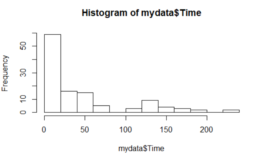
I’m modelling some data on reaction times, and I want to do some initial examination of my data, to pick the right distribution. For this, I usually calculate the residuals of my model, plot them and check QQ-plots of the residuals.

However, when I calculate the residuals using:

residuals(mod1)

My resulting plots show that the residual estimated errors are all above zero, and none of them are even close to zero. What could be causing this?

The code I run is as follows, and I’ve added a least replicable example of my data.
Final_example.csv (4.2 KB)

mydata<-read.csv("Final_example.csv",rownames=FALSE,header=TRUE,na = "-")
mydata$Time=as.numeric(as.character(mydata$Time))
mydata$GC=as.factor(mydata$Ground_XCAZNOPY)
mydata$Block=mydata$Block
mydata$Plant=as.factor(mydata$Plant)
mydata$BA=as.factor(mydata$BA)
mydata$Vegetation=as.factor(mydata$Vegetation)
mydata$Food=as.factor(mydata$Food)

mod1<-brm(Time~BA+GC+Food+Plant+Vegetation+(BA:GC)+(BA:Food)+(BA:Plant)+(GC:Food)+(1|Block),data=mydata)
res<-residuals(mod1)
plot(res)
qqnorm(res)
qqline(res)

The residual plot and QQ-plot is also attached here.

[JLC]

How do things look if you use a gamma distribution rather than Gaussian?

[IdaC]

I get errors if I use a gamma distribution with link = inverse:

Chain 1: Rejecting initial value:
Chain 1: Error evaluating the log probability at the initial value.
Chain 1: Exception: gamma_lpdf: Inverse scale parameter[1] is -1.72645, but must be > 0! (in ‘model324c750db2e_153aca50ee007d54c9db5786abc59841’ at line 56)

But if I change it to link = log, I get the following plots:

[JLC]

I don’t think the assumption of normally distributed residuals applies to gamma GLM’s. I seen instead seen recommendations for QQ Plots of residuals against a simulation-based expected distribution.

How do your posterior predictive checks look?

[IdaC]

When I use pp_check, I get the following plots:

For the Gaussian distribution:

For the Gamma (link = log) distribution:

[JLC]

After you able to share your model and some example data?

[IdaC]

I already did, everything is in the first post.

[JLC]

Apologies! I should refrain from posting before coffee!

The PPC suggests Gaussian isn’t a good fit for the data and that gamma is doing a reasonable job.

You could also look at predictor-specific ppc’s with:

pp_check( Mod1, type = "dens_overlay_grouped", group = "BA")

[mike-lawrence]

Any obvious explanation for that bump at 140?

[JLC]

I did a little re-arranging

## Required packages
Pkgs <- c("tidyverse", "brms", 
          "rstan", "bayesplot", 
          "parallel", "cmdstanr")

### Load packages ====
lapply(Pkgs, require, c = T)


## Set computing options ====
ncores = detectCores()

### Create data frame
mydata <- read.table("Final_example.csv",header=TRUE,na = "-", sep = ";") %>%
        mutate(Time = as.numeric(Time),
               BA = factor(BA),
               GC = factor(Ground_XCAZNOPY),
               Block = factor(Block),
               Plant = factor(Plant),
               Vegetation = factor(Vegetation),
               Food = factor(Food)
               ) %>%
        select(-Ground_XCAZNOPY)

Range of outcome:
range(mydata$Time, na.rm = T)
[1] 10 230

Default model:

mod1 <- brm(Time ~ BA + 
                    GC + 
                    Food +
                    Plant +
                    Vegetation + 
                    BA:GC +
                    BA:Food +
                    BA:Plant +
                    GC:Food +
                    (1|Block),
            data = mydata,
            family = Gamma(link = "log"),
            #prior = priors,
            inits = "random",
            iter = 2000,
            warmup = 1000,
            chains = 4,
            cores = ncores,
            sample_prior = TRUE,
            save_pars = save_pars(all = TRUE),            
            backend = "cmdstan", # You can comment this line out if you don't have cmdstan
            normalize = FALSE, # This should be commented out if you aren't using cmdstan
            control = list(max_treedepth = 12,
                           adapt_delta = 0.9))

Some PPC’s

pp_check(mod1, type = "dens_overlay_grouped", group = "BA")
pp_check(mod1, type = "dens_overlay_grouped", group = "GC")
pp_check(mod1, type = "dens_overlay_grouped", group = "Food")
pp_check(mod1, type = "dens_overlay_grouped", group = "Plant")
pp_check(mod1, type = "dens_overlay_grouped", group = "Vegetation")
pp_check(mod1, type = "dens_overlay_grouped", group = "Block")

LOO evaluation
loo(mod1)

Computed from 4000 by 118 log-likelihood matrix

         Estimate   SE
elpd_loo   -586.5 19.9
p_loo        23.7  8.3
looic      1173.0 39.9
------
Monte Carlo SE of elpd_loo is NA.

Pareto k diagnostic values:
                         Count Pct.    Min. n_eff
(-Inf, 0.5]   (good)     114   96.6%   612       
 (0.5, 0.7]   (ok)         1    0.8%   1632      
   (0.7, 1]   (bad)        1    0.8%   111       
   (1, Inf)   (very bad)   2    1.7%   3         

I get a number if divergences, likely from using default (relatively flat) priors for all parameters. Do you have some ideas to constrain the estimates?

[IdaC]

I’m not completely sure, but this is the Histogram of my response variable, Time, and there is a clear peak at about 10, and then again at around 140, so that might be the explanation. So the distribution kind of has two peaks.

[mike-lawrence]

I meant a theoretical explanation, from the perspective of your subject matter expertise.

[IdaC]

Oh, sorry. It makes a lot of sense (for my experiment), that the subjects either have a very fast or a very slow reaction, while very few will be in between. So to some degree it fits the “theory” quite well, but not as to why 140 pops out, as it could just as well have been 200.

[JLC]

Adding SubjectID as a grouping variable might help tighten up the estimates for individuals.

[mike-lawrence]

@IdaC

subjects either have a very fast or a very slow reaction, while very few will be in between.

If there are multiple observations for each subject and within a subject some of those observations are going to be fast while some are going to be slow, even accounting for all the other predictors, then you’ll need to use a mixture model on top of the structure you already have.

If there are not multiple observations per subject, and merely multiple subjects each of which might be either fast or slow, then it’s possible @JLC’s suggestion to add subjectID (n.b. must be a factor label, not a numeric label) as a grouping variable might help (@JLC: in brms world is “adding as a grouping variable” the same as specifying subjectID as a random effect?). However, if you expect fast and slow subjects even accounting for all the predictors, then a mixture model will account for that better.

[JLC]

Yep! SubjectID as a grouping variable is done by entering it as a random intercept (1|SubjectID). But, if this is a repeated measures design, it might also be worthwhile to look at the correlations between other predictors for each subject (i.e., a random slope: (1|SubjectID) + (0 + BA + GC|SubjectID)).

I was also thinking mixture model to separate the slow vs fast times/processes would be worth a look.

[IdaC]

Ok, I can add subjectID, but just as you say, it’s a repeated measures design, so the same subjects are tested twice. I’ve never tried Bayesian mixture models, but I’ll try and look into that :-) Do you have any literature on the subject that you can recommend?

[mike-lawrence]

The User Guide has a section on mixture models, but it wouldn’t surprise me if @paul.buerkner (tagging to see if he can confirm) had mechanisms for specifying the kind of mixture you need in brms too.

[JLC]

Hopefully Paul can add some insight!

Mixture models are tough to get working well. Below is a general example, but note that it doesn’t work very well at all. Prior specification is pretty important, so I added in a couple of lines to demonstrate how you can see the available priors.

## Specify the mixtures
mix <- mixture(Gamma(link = "log"), Gamma(link = "log"), order = "mu")

## Specify the model formula
Mix_fmla <- bf(Time ~ BA + 
                      GC + 
                      Food +
                      Plant +
                      Vegetation + 
                      BA:GC +
                      BA:Food +
                      BA:Plant +
                      GC:Food +
                      (1|Block),
                    center = TRUE) 

# Get list of possible priors
Mix_list <- get_prior(Mix_fmla,
                      data = mydata,
                      family = mix) 

## Run model
Mix_Mod <- brm(
  Mix_fmla,
  data = mydata,
  family = mix, 
  #prior = Mix_priors, # This is where you would specify your priors
  inits = "random",
  iter = 2000,
  warmup = 1000,
  chains = 4,
  cores = ncores,
  sample_prior = TRUE,
  save_pars = save_pars(all = TRUE),
  backend = "cmdstan", # You can comment this line out if you don't have cmdstan
  normalize = FALSE, # This should be commented out if you aren't using cmdstan
  control = list(max_treedepth = 12,
                 adapt_delta = 0.9)
)

[IdaC]

Thanks! I just found the “Finite Mixture families in brms” and it actually explains it pretty well, so I’m trying it out (same code as you wrote though, so thank you!) :-)