I’m trying to model the bicycle count data from the table in the exercises of Chapter 3 of Bayesian Data Analysis by Gelman et. al. using a hierarchical binomial model with population effects for street type and the presence of a bike route.
Every time I sample the posterior (using rstan 2.18.2) I get very different results for the final probabilities of seeing bikes in each city block. I’ve tried extracting a huge number of samples each run (about 1.1 million) and the results are still just as variable.
Is there something pathological in the posterior that’s causing this? Or perhaps the model itself is ill-posed? How would I go about diagnosing this situation?
Below is my Stan code as well as self-contained R code to generate a plot of the raw proportions of bikes to total traffic versus the estimates from the model. I’ve also included two examples of those plots at the end showing the variation in results.
data{
    int<lower=1> N;
    int bikes[N];
    int total[N];
    int is_fairlybusy[N];
    int is_busy[N];
    int bike_route[N];
    int block_id[N];
}
parameters{
    vector[N] a_bl;
    real a;
    real a_fair;
    real a_busy;
    real b;
    real<lower=0> sigma;
}
model{
    vector[N] p;

    // fixed priors
    sigma ~ gamma(2, 2);
    b ~ normal(1, 10);
    a ~ normal(-2, 10);
    a_fair ~ normal(0, 10);
    a_busy ~ normal(0, 10);

    // adaptive prior
    a_bl ~ normal(0, sigma);

    // model
    for ( i in 1:N ) {
        p[i] = a + a_bl[block_id[i]] + a_fair*is_fairlybusy[i] + a_busy*is_busy[i] + b*bike_route[i];
    }

    // likelihood
    bikes ~ binomial_logit(total, p);
}
library(rstan)
bike_data <- data.frame(
bikes = as.integer(c(16, 9, 10, 13, 19, 20, 18, 17, 35, 55, 12, 1, 2, 4, 9, 7, 9, 8, 8, 35, 31, 19,
38, 47, 44, 44, 29, 18, 10, 43, 5, 14, 58, 15, 0, 47, 51, 32, 60, 51, 58, 59,
53, 68, 68, 60, 71, 63, 8, 9, 6, 9, 19, 61, 31, 75, 14, 25)),
other = as.integer(c(58, 90, 48, 57, 103, 57, 86, 112, 273, 64, 113, 18, 14, 44, 208, 67, 29, 154,
29, 415, 425, 42, 180, 675, 620, 437, 47, 462, 557, 1258, 499, 601, 1163, 700,
90, 1093, 1459, 1086, 1545, 1499, 1598, 503, 407, 1494, 1558, 1706, 476, 752,
1248, 1246, 1596, 1765, 1290, 2498, 2346, 3101, 1918, 2318)),
is_fairlybusy = as.integer(c(rep(0, 18), rep(1, 20), rep(0, 20))),
is_busy = as.integer(c(rep(0, 38), rep(1, 20))),
bike_route = as.integer(c(rep(1, 10), rep(0, 8), rep(1, 10), rep(0, 10), rep(1, 10), rep(0, 10)))
)
bike_data$total <- bike_data$bikes + bike_data$other
bike_data$block_id <- 1:nrow(bike_data)
fit <- stan(
model_code = model_code,
data = list(
N = nrow(bike_data),
bikes = bike_data$bikes,
total = bike_data$total,
is_fairlybusy = bike_data$is_fairlybusy,
is_busy = bike_data$is_busy,
bike_route = bike_data$bike_route,
block_id = bike_data$block_id
),
iter = 1e4,
warmup = 2e3,
chains = 4,
cores = 4,
control = list(max_treedepth = 15)
)
samples <- extract(fit)
logit_block <- sapply(1:58, function(i) samples$a + samples$a_bl[,i])
logit_residential <- sapply(
1:18,
function(i) logit_block[,i] + ifelse(i <= 10, samples$b, 0)
)
logit_fairlybusy <- sapply(
19:38,
function(i) logit_block[,i] + samples$a_fair + ifelse(i <= 28, samples$b, 0)
)
logit_busy <- sapply(
39:58,
function(i) logit_block[,i] + samples$a_busy + ifelse(i <= 48, samples$b, 0)
)
# any inverse logit function will do
residential <- brms::inv_logit_scaled(logit_residential)
fairlybusy <- brms::inv_logit_scaled(logit_fairlybusy)
busy <- brms::inv_logit_scaled(logit_busy)
residential_mu <- apply(residential, 2, mean)
fairlybusy_mu <- apply(fairlybusy, 2, mean)
busy_mu <- apply(busy, 2, mean)
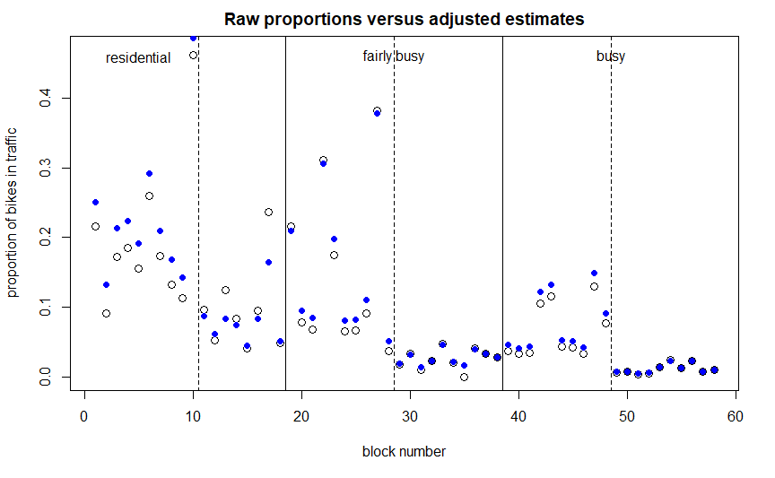
plot(
1:58, bike_data$bikes/bike_data$total,
cex = 1.2,
ylim = c(0, 0.47),
xlab = "block number", ylab = "proportion of bikes in traffic",
main = "Raw proportions versus adjusted estimates",
)
points(1:58, c(residential_mu, fairlybusy_mu, busy_mu), pch = 16, col = "blue")
lines(c(18.5, 18.5), c(-0.02, 0.49))
lines(c(38.5, 38.5), c(-0.02, 0.49))
lines(c(10.5, 10.5), c(-0.02, 0.49), lty = 2)
lines(c(28.5, 28.5), c(-0.02, 0.49), lty = 2)
lines(c(48.5, 48.5), c(-0.02, 0.49), lty = 2)
text(5, 0.46, "residential")
text(28.5, 0.46, "fairly busy")
text(48.5, 0.46, "busy")
In these plots the open circles correspond to raw proportions (bikes/total) and the blue dots correspond to model estimates. Street types are separated with solid vertical lines, and within each street type the estimates corresponding to bike routes and non bike routes are separated by dashed vertical lines (with bike routes on the left of the dashed lines).