Using GP for autocorrelation in a time-series model: memory pressure, GP kernel definition

Real quick, I’ll respond to the other stuff in a bit, but

f = L * z + L being the Cholesky factor of a covariance of an RBF + z ~ normal(0, 1) implies that the prior on f is f ~ multi_normal(0, rbf_covariance)

So you don’t need g ~ normal(f, sigma_gp);

There are two hyperparameters of the RBF GP, one corresponding to the input scale (length scale, or rho in the manual) and one corresponding to the output scale (alpha in the manual). You can keep alpha outside the Cholesky – if that makes sense? Like, you can do the Cholesky assuming alpha = 1 and then scale the Cholesky as you like to still sample sigma. I’m probably not saying that clearly… Anyway, the thing you probably want is this:

transformed parameters {
  vector[N] g = L * z * sigma_gp; // non-centered parameterization;
}

Along with z ~ normal(0, 1) to do the GP, and then get rid of g as an extra random variable.

Full modified model:

data {
  int<lower=1> N; // number of (time) points in series
  matrix[N,N] L;

  int<lower=0> K; // number of predictos
  matrix[N, K] X; // predictor design matrix
  vector[N] response; // vector of Alongshore current speeds

//prediction
  int<lower=1> S; // length of wind series to simulate over
  int<lower=0> sK; // number of predictors for simulation
  matrix[S, sK] SIM; // matrix of ismulated values

}
parameters {
  vector[K] B; // coefficients of the model (both intercepts and slopes)
  vector[N] z;
  real<lower=0> sigma_response;
  real<lower=0> sigma_gp;
  real<lower=0> inv_rho_sq;
}
transformed parameters {
  vector[N] g = L * z * sigma_gp; // non-centered parameterization;
}
model {
    vector[N] mu;
    B[1] ~ normal(0,1); // intercept prior
    B[2:K] ~ normal(0,1); // slope priors
    g ~ normal(0, 1);
    z ~ normal(0, 1);
    sigma_response ~ normal(0, 1);
    sigma_gp ~ normal(0, 1);
    mu = X * B + f ;
    response ~ normal(mu, sigma_response);
}
generated quantities{
  vector[S] sim_cur; //simulated response output
  vector[N] mu_pred;
  vector[N] pred_cur;
  vector[N] log_lik;
  vector[N] resids;
    sim_cur = SIM * B; // simulated response across the range of params
    mu_pred = X*B + g; //+ approx_L(M, scale, Distance, inv_rho_sq) * g;
  for(i in 1:N){
    pred_cur[i] = normal_rng(mu_pred[i], sigma_response); // posterior predictions of the model
    log_lik[i] = normal_lpdf(response[i] | mu_pred[i], sigma_response); // compute log likelihood for us in AIC 
  }  
  resids = response - mu_pred;
}

Hahaha yeah, +1

That’s happened to me before as well. I like to try to to think of the GP as an extra thing that just comes in and explains what’s left over, but it just never works out that well. The GP can explain just about anything.

Check pairplots on these parameters too. It’s possible things are unidentified, and since the GP might just be explainin’ things, then these things could get twisted up with the GP too.

Looking at the original plot (first post), it looks like the effect of the red thing on the black thing could be really small, if it’s there. I guess we know wind influences ocean current speeds in some way though? What are your thoughts here? Could the influence you’re trying to detect be small? If it is, there might be a way to play around with simulated data to get an idea of the resolution of this method? (I’m not sure – that’s why I ended the sentence with a question mark haha)

Additionally to what you said, Ben (very helpful source for this and future problems):

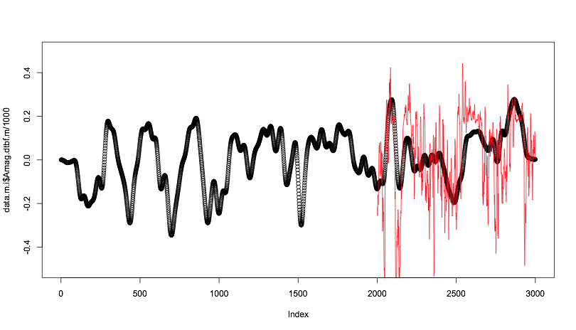
If we look at the first graphic, there is hardly a common trend between both graphs, at least I don’t see any.
However in the differences of both series (1st derivative). That’s why the model I posted, respects the relationship between wind and currents with a correlation between two GPs. They share some variation, although not a relationship in their means.

Second one may try also a period Kernel for the GP, although I’ve no idea about approximations. But parallel + GPU is on track, so we can hope for speedups.

Your observations are valid. However that first graph sucks because I was apparently too lazy to put the series on the same units. It makes things difficult to see. Here is a better version.

Alongshore wind stress in blue. Alongshore currents (filterd) in black.

Here’s a scatterplot with the same two series:

And here is the same basic layout but with the first-order difference of each series, though it isn’t very useful because of the noise in the wind.

Here’s a scatterplot of the first-order differences:

So I think the influence that I am trying to tease out is not exactly small, but it has the problem of being more impactful under a subset of conditions. When the wind is strong, it is the main driver of the currents. When the wind is weak, it is not the main driver of the currents and the model doesn’t have much information to go on. However, my hope was to deal with the latter problem by allowing some lag in the model (either through the inclusion of moving averaged/lagged predictors or through varying length scales in a GP), because if you know how currents were flowing and wind was blowing for a while before the wind shuts off, you know something about what the currents are going to do when the wind does shut off.

In the real-world, this is because the coastal basin is kind of like a giant bathtub; under windy conditions the water gets piled up at one end of the tub and when the wind relaxes, that water sloshes back the other direction. So the wind shuts off, but the strength of the response in terms of rate and magnitude depends on how much water got piled up, because in the absence of wind it is now simply the pressure gradient force from having a tilted fluid that is driving currents. This is a fundamental process but difficult to capture because the bathtub is of course impossibly complex in shape and is open to the rest of the ocean processes.

So I’m not sure if that helps clarify things any further, but I hopefully have filled in some of the gaps.

I am looking at that paper you linked, Andre, (http://iopscience.iop.org/article/10.1088/1367-2630/15/5/053024/pdf) and trying to come up with a way to fit my data to a physical model to be more explicit. Again, if I can get to a point where I can predict the coastal jet from the widely available wind data, then I am one step closer to the goal of hindcasting the eddy index. So I will try to use the model and some error term and fit it to my data.

I am trying to run your Kalman model with the full data set and M = 10 basis functions retained, but it is just not getting anywhere on my computer which is a respectable performing but not very new Macbook pro. I see now what you are saying with using two GPs in there and it makes good sense. I just wish I could fit that!

As for @bbbales2 model, I have also tried to fit that with all the data after having made those changes you suggested, but again just suffering from computational costs. I have been playing with the INLA methods and they seem interesting, but the ARIMA stuff just won’t work on these data because the lags go so far and it just fails to fit when I try to do high-order differencing. So I might be able to get something useful out of the matern2d or the random-walks, but I’m not sure yet whether those are valid formulations (or how to use that package to generate predictions and get posteriors, etc.).

I will see about doing a long long run on the desktop PC at my lab or trying to get some core time at the campus computer or NSF XSEDE, but while those free me from constantly running my processor at the max, I don’t think they will really speed things up terribly.

I’ll keep you updated on these attempts! Thanks for your help so far. Feel free to shoot any other ideas out there. I promise to some day write this up in a coherent post for future Stan users (or abusers… I’m not sure what title I’ve earned). These models are all useful and interesting in their own right… just need to address the modeling problem without slamming into the computational limits.

I wonder if this has something to do with the scale parameters going into the GP? It would be really interesting to take a look at the sensitivity to priors. I wonder if you can somehow weight the GP over the linear predictors if you use really uninformative priors.

Anyway, this result just has me thinking. I’ll try to come up with a way to formulate the model that is more similar to Andre’s- accounting for measurement error in the winds and currents and then relating the two according to some correlation. Between that and the fixed length scale method, it might just work.

Oooh oooh question time!

Is there a way to get the information you’re looking for from a plain ol’ regression?

What is the information you’re looking for here (if that’s not too big a question)?

What’s the importance of the time series here?

If the GP fits (and I think we have a vague idea of what a ‘fit’ would look like, right?), then what do we learn?

(if we can think of excuses to ditch the GP then we can fix your computational problems :P)

Perhaps plain old regression is fine. The whole GP approach came from a desire to model autocorrelation. The time series of the predictor and response are significantly autocorrelated out to a high number of lags, so traditional ARIMA type models seemed insufficient to me. So I went on to look for other ways to deal with the influence of autocorrelation.

Ultimately, all I really want to know is how the wind, both most recently and the accumulation of wind as represented by moving averages, affects current speeds at this location (or, perhaps more accurately, what the relationship between wind speeds and current speeds is at this location). Then I want to do the same thing with the principal component that describes an eddy index. That way my whole story can go from wind, the driving force, to eddy circulation by way of the effect of wind on the coastal current.

What do you think? Can we just ignore autocorrelation and model this as a simple linear regression?

@bbbales2 Hey Ben, I have a quick question for you. When I wrote the model to use a fixed length scale and a pre-computed cholesky, I went back to computing the covariance matrix with the straight squared exponential:

I wonder if I am screwing up the distance matrix Dmat. I was inputting an N x N matrix where column i consists of distances in time centered on row i (so the zero point is the observation in time).

Dmat <- matrix(rep(1:length(time), each = length(time)), nrow = length(time), ncol = length(time))
for(i in 1:nrow(Dmat)){
	Dmat[i,] <- Dmat[i,] - i
}
Dmat <- t(Dmat)
> head(stan_data_i$Distance)
     [,1] [,2] [,3] [,4] [,5] [,6] [,7] [,8] [,9] [,10] [,11] [,12] [,13] [,14] [,15] [,16] [,17] [,18] [,19] [,20] [,21] [,22] [,23] [,24] [,25] [,26]
[1,]    0   -1   -2   -3   -4   -5   -6   -7   -8    -9   -10   -11   -12   -13   -14   -15   -16   -17   -18   -19   -20   -21   -22   -23   -24   -25
[2,]    1    0   -1   -2   -3   -4   -5   -6   -7    -8    -9   -10   -11   -12   -13   -14   -15   -16   -17   -18   -19   -20   -21   -22   -23   -24
[3,]    2    1    0   -1   -2   -3   -4   -5   -6    -7    -8    -9   -10   -11   -12   -13   -14   -15   -16   -17   -18   -19   -20   -21   -22   -23
[4,]    3    2    1    0   -1   -2   -3   -4   -5    -6    -7    -8    -9   -10   -11   -12   -13   -14   -15   -16   -17   -18   -19   -20   -21   -22
[5,]    4    3    2    1    0   -1   -2   -3   -4    -5    -6    -7    -8    -9   -10   -11   -12   -13   -14   -15   -16   -17   -18   -19   -20   -21
[6,]    5    4    3    2    1    0   -1   -2   -3    -4    -5    -6    -7    -8    -9   -10   -11   -12   -13   -14   -15   -16   -17   -18   -19   -20

Now I’m not sure if that is the right way of doing it at all. Maybe I’m screwing that up?

d <- as.matrix(dist(time,upper=TRUE))**2
does the same and is more short. Not using normalization and centering
might result in a length-scale with a wide range.

Keep it simple. As simple as possible, but not simpler.
A. Einstein.

Can you come up with the most simple useful model and develop from
there?

m1 <- lm(Amag.dtbf.m/1000 ~ scale(aspe.1hr.tau.x) , data = data.m.i[1:2000,])

currents @ 1 hr ~ winds @ 1 hr

Fit to the first 2000 points and predicting the remaining points.

It’s really not all that bad.

2 Likes

Try with adding autocorrelation too, since you mentioned you want to it. Becoming a little bit Stan offtopic
now.

m2 <- lm(Amag.dtbf.m[-1]/1000 ~ scale(aspe.1hr.tau.x[-1]) + Amag.dtbf.m[-2000] , data = data.m.i[1:2000,])

Looks reasonable to me, but if you’re scared of bugs, you can either write out the covariance matrix explicitly:

x = matrix(0, nrow = N, ncol = N)

for(i in 1:N) {
  for(j in 1:N) {
    x[i, j] = exp(-((x[i] - x[j])^2) / (2 * l^2));
  }
}

Maybe it’s slow in R but whatever.

Or you can do these calculations in the transformed data block in your Stan model and just use the built in cov_exp_quad n’ such. This way at least if you write bugs you can have some confidence you’re consistently writing bugs cause it’s just copy paste haha.

Like:

transformed data {
   matrix[N, N] x = cov_exp_quad(...);
   ...
}

The transformed data block only runs once so you’re safe efficiency-wise.