Two-Tier or Testlet-IRT Model in brms

Dear readers,
I want to implement an IRT testlet model and a kind oftwo-tier model (see Cai, 2010; https://link.springer.com/article/10.1007/s11336-010-9178-0) as an extention to that in brms. I wonder if this is possible in brms and how the corresponding formula might look. Let’s begin with a quick overview on my data structure.

I use a dataset of 74 items with 575 persons answering these items. The items are nested in testlets because they have to make multiple decissions (answer multiple items) to each of 17 item stems. The item stems can be assigned to different primary factors (one of three) in theory.

For a unidimensional 1PL model I came up with the following code:

formula_PCK_1D_1pl <- bf(
  response ~ 1 + (1 | item) + (1 | ID) + (0 + testlet_char | ID),
  family = brmsfamily("bernoulli", link = "logit")
)

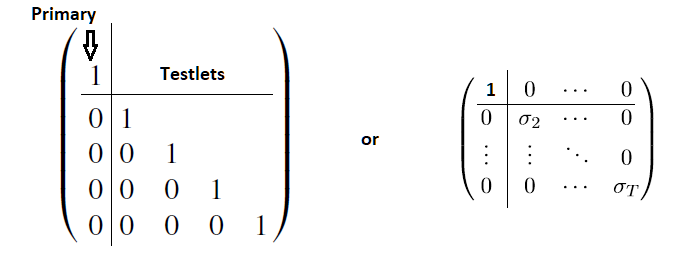
The testlet assignment is given by an string. My problem is that I have to define a special covariance structure towards the model. In the unidimensional case it should have diagonal form. So there should be no correlation between the testlet factors and the testlet factors with the primary factor. Using the || operator semms not to set the correlation to 0 but just doesn’t calculate the cor, right?

I wondered if I could do something appropriate with the fcor term? Or setting lkj(100) to get at least very low correlations? How can I set up correlation between (1 | ID) and the (0 + testlet_char | ID) terms?

For a 3PL multidimensional model (where each item is assigned to exactly a single primary factor/dimension) I tried:

formula_PCK_3D_3pl <- bf(
response ~ gamma + (1 - gamma) * inv_logit(beta + exp(logalpha) * theta + testlet),
  nl = TRUE,
  theta ~ 0 + (0 + dimension_char | ID),
  beta ~ 1 + (1 | item),
  logalpha ~ 1 + (1 | item),
  logitgamma ~ 1 + (1 | item),
  nlf(gamma ~ inv_logit(logitgamma)),
  testlet ~ 0 + (0 + testlet_char | ID)
  family = brmsfamily("bernoulli", link = "identity")
)

Am I on the right way? Can you help me an formula for a dataset with, lets say, four different testlets?

Right now even the 1PL unidimensional models needs a huge amount of time to finish. I tried code for the rstan package as well which finishes much faster but doesn’t show convergance (for the code used see Luo et Jiao, 2018; https://www.ncbi.nlm.nih.gov/pmc/articles/PMC6096466/). The modles via ML (mirt::bfactor, TAM::tam.fa) converged well for up to 2PL already.

  • Operating System: Win 10x64 1909
  • brms Version: 2.13.5

Sincerely, Simon

1 Like

Welcome to the Stan forums!

|| sets the correlation parameter to zero, which is likely what you want. to set up correlations between different random effects terms, use brms ID syntax (see https://journal.r-project.org/archive/2018/RJ-2018-017/index.html for example). In your case, it would be (1 | i | ID) + (0 + testlet_char | i | ID), where “i” is arbitary.

the 3PL models looks reasonable, but I cannot evaluate it with respect to the testlet details.

The fact that such models take time is to be expected. A few hours are likely.

1 Like

Ah. That’s great. I’ve seen the |i| in your examples for 3Pl for the item parameters before. Wasn’t sure if it will be the correct thing for the nested terms as well. I wasn’t sure, if || means cor is not computed or fixed to zero. Thanks for your explaination.

How can I set the correlation established with |i| to zero? Or should I just don’t use |i| and the correlation will be set to zero as well?

I am afraid I don’t understand your question. If you use || the correlation will be set to zero. If you use | or |i| you will estimate correlations. If you have two terms with | the random effects in different terms will have correlations fixed to zero.

It might be a conceptional problem in my understanding. I want to set the covariance matrix to:

Covarianz

So neither the testlet factors are correlated with each other nor they are correlated with the primary factor. They should all be orthogonal to each other. At least in the 1PL model the variace can differ from 1 (on the diagonal). In the 2PL model I might implement this by adding an additional alpha term to the testlet term (see generalized Testlet model at Curtis, 2010; https://www.jstatsoft.org/index.php/jss/article/view/v036c01/v36c01.pdf).

So in my mind it seems to be a difference between: a) parameteres are estimated so that correlation gets zero (so correlation might has to be computed to check this?)
and b) correlation isn’t computed at all (and thus could differ from zero).

But maybe c) is correct? correlation not modeled means correlation is zero. (Because of the used form of matrices?)

Because in my mind a) is dominant, I asked how I can set correlation(primary factor : (1 | ID), testlet_i) = 0 and to do that I thought I have to specifiy the correlation via |i| first to set it 0 afterwards.

1 Like

You have a misconception here. You want to assume the correlation to be zero, which is what || does for you. If you think of it from a Bayesian perspective, the correlation matrix is part of a prior. Whatever the prior assumes does not have to be reflected in the posterior, and you will see this in both bayesian and frequenst estimates of the obtained factor scores. That is, they will still correlate no matter what you force the correlation to be. Estimating the correlation and then fixing it to zero via a prior is equivalent to not modeling the correlation in the first place via ||. I know our minds are clouded from what we have learned in frequentist statistics, but there really is no difference in (a) and (b) given that your prior on the correlation in (a) forces it to zero.

Okay. So if I dont use the |i| term this would be closer to the prior information, that the primary factor and the testlet factors are orthogonal. And in the end I will see if the posterior parameters will give me a correlation close to zero, right? (I think here roots my suggestion to set a very high value for lkj() so the posterior is closer to the prior values.)

Anyway, when I modeled the correlation I found that zero was in the 95 % confidence intervall for all correlation but 2. That is already close to my prior assumption. (In contrast modeling the multiple dimensions gave clear non zero correlations.)

So maybe I check the posterior correlations in the || model and compare these. And maybe in a model that links the testlets to the primay dimension als well via |i|. I’ll use the time this model runs to check if i can find a neat Bayesian way to use my samples for correlation estimation instead of the point estimates.

Thanks for your help so far. Your work is awesome!

Yes(ish). We have two correlations here.

One is the correlation parameter. If you use ||, this correlation parameter is 0. If you estimate the parameter with lkj(100) (say), the correlation parameter will also be very close to zero.

The other correlation is the empirical correlation between estimated factor scores, which can be wildly different from zero no matter what you do with the correlation parameter.

Dear readers,
I came across another problem with my model specification. One of the items in the test has a testlet size of 1 (or isn’t neted in a testlet at all). The specification

testlet ~ 0 + (0 + testlet_char | ID)

therefore interfers with the theta for this item term. You can see the effect in the PSIS plot.

Is there a way, to set the term to zero in this case? I fear setting testlet_char to NA for this item will remove it from the analysis but I haven’t come up with a idea yet since I can only set a prior for testlets sd nor interceps. I hope you can help me here as well.

1 Like

I’ve came up with a promising solution:
Setting the prior for the SD of the testlet to constant(0) resulted in a PSIS plot without high k values for all observations for a single item and set the theta values to 0 for all persons. This corresponds to my expectations how the model should behave for items without a testlet group.

Unfortunately: the beta parameter estimates are now far off compared to mirt::bfactor, TAM::fa or sirt::mcmc.3pno.testlet (restricted slopes and guessing). The old estimates (where SD for Testlet 8 weren’t restricted) are very close to the other functions.

So setting SD for a testlet 0 seems not to be the right way. Do you have a suugestion how to set a testlet effect to zero for some items @paul.buerkner? Is here a way to state this in brms or do I have to hack the rstan code?

In the rstan code (see below) I would try setting the vector[N] Z_3_testlet_31; or vector[N_3] r_3_testlet_31; to zero. (I’m unsure here, but I tend to set the vector[N] Z_3_testlet_31; because the vector[N_3] r_3_testlet_31; is calculated based on vector[N] Z_3_testlet_31;. Is this assumption right?)

Edit: I followed the BUGS-Code (found here: https://www.jstatsoft.org/article/view/v036c01) and changed the Testletnumber for items without testlet to n_testlets+1 = 31.

// generated with brms 2.13.5
functions {
}
data {
  int<lower=1> N;  // number of observations
  int Y[N];  // response variable
  int<lower=1> K_beta;  // number of population-level effects
  matrix[N, K_beta] X_beta;  // population-level design matrix
  // data for group-level effects of ID 1
  int<lower=1> N_1;  // number of grouping levels
  int<lower=1> M_1;  // number of coefficients per level
  int<lower=1> J_1[N];  // grouping indicator per observation
  // group-level predictor values
  vector[N] Z_1_theta_1;
  // data for group-level effects of ID 2
  int<lower=1> N_2;  // number of grouping levels
  int<lower=1> M_2;  // number of coefficients per level
  int<lower=1> J_2[N];  // grouping indicator per observation
  // group-level predictor values
  vector[N] Z_2_beta_1;
  // data for group-level effects of ID 3
  int<lower=1> N_3;  // number of grouping levels
  int<lower=1> M_3;  // number of coefficients per level
  int<lower=1> J_3[N];  // grouping indicator per observation
  // group-level predictor values
  vector[N] Z_3_testlet_1;
  vector[N] Z_3_testlet_2;
  vector[N] Z_3_testlet_3;
  vector[N] Z_3_testlet_4;
  vector[N] Z_3_testlet_5;
  vector[N] Z_3_testlet_6;
  vector[N] Z_3_testlet_7;
  vector[N] Z_3_testlet_8;
  vector[N] Z_3_testlet_9;
  vector[N] Z_3_testlet_10;
  vector[N] Z_3_testlet_11;
  vector[N] Z_3_testlet_12;
  vector[N] Z_3_testlet_13;
  vector[N] Z_3_testlet_14;
  vector[N] Z_3_testlet_15;
  vector[N] Z_3_testlet_16;
  vector[N] Z_3_testlet_17;
  vector[N] Z_3_testlet_18;
  vector[N] Z_3_testlet_19;
  vector[N] Z_3_testlet_20;
  vector[N] Z_3_testlet_21;
  vector[N] Z_3_testlet_22;
  vector[N] Z_3_testlet_23;
  vector[N] Z_3_testlet_24;
  vector[N] Z_3_testlet_25;
  vector[N] Z_3_testlet_26;
  vector[N] Z_3_testlet_27;
  vector[N] Z_3_testlet_28;
  vector[N] Z_3_testlet_29;
  vector[N] Z_3_testlet_30;
  vector[N] Z_3_testlet_31;
  int prior_only;  // should the likelihood be ignored?
}
transformed data {
}
parameters {
  vector[K_beta] b_beta;  // population-level effects
  vector<lower=0>[M_1] sd_1;  // group-level standard deviations
  vector[N_1] z_1[M_1];  // standardized group-level effects
  vector<lower=0>[M_2] sd_2;  // group-level standard deviations
  vector[N_2] z_2[M_2];  // standardized group-level effects
  vector<lower=0>[M_3] sd_3;  // group-level standard deviations
  vector[N_3] z_3[M_3];  // standardized group-level effects
}
transformed parameters {
  vector[N_1] r_1_theta_1;  // actual group-level effects
  vector[N_2] r_2_beta_1;  // actual group-level effects
  vector[N_3] r_3_testlet_1;  // actual group-level effects
  vector[N_3] r_3_testlet_2;  // actual group-level effects
  vector[N_3] r_3_testlet_3;  // actual group-level effects
  vector[N_3] r_3_testlet_4;  // actual group-level effects
  vector[N_3] r_3_testlet_5;  // actual group-level effects
  vector[N_3] r_3_testlet_6;  // actual group-level effects
  vector[N_3] r_3_testlet_7;  // actual group-level effects
  vector[N_3] r_3_testlet_8;  // actual group-level effects
  vector[N_3] r_3_testlet_9;  // actual group-level effects
  vector[N_3] r_3_testlet_10;  // actual group-level effects
  vector[N_3] r_3_testlet_11;  // actual group-level effects
  vector[N_3] r_3_testlet_12;  // actual group-level effects
  vector[N_3] r_3_testlet_13;  // actual group-level effects
  vector[N_3] r_3_testlet_14;  // actual group-level effects
  vector[N_3] r_3_testlet_15;  // actual group-level effects
  vector[N_3] r_3_testlet_16;  // actual group-level effects
  vector[N_3] r_3_testlet_17;  // actual group-level effects
  vector[N_3] r_3_testlet_18;  // actual group-level effects
  vector[N_3] r_3_testlet_19;  // actual group-level effects
  vector[N_3] r_3_testlet_20;  // actual group-level effects
  vector[N_3] r_3_testlet_21;  // actual group-level effects
  vector[N_3] r_3_testlet_22;  // actual group-level effects
  vector[N_3] r_3_testlet_23;  // actual group-level effects
  vector[N_3] r_3_testlet_24;  // actual group-level effects
  vector[N_3] r_3_testlet_25;  // actual group-level effects
  vector[N_3] r_3_testlet_26;  // actual group-level effects
  vector[N_3] r_3_testlet_27;  // actual group-level effects
  vector[N_3] r_3_testlet_28;  // actual group-level effects
  vector[N_3] r_3_testlet_29;  // actual group-level effects
  vector[N_3] r_3_testlet_30;  // actual group-level effects
  vector[N_3] r_3_testlet_31;  // actual group-level effects
  r_1_theta_1 = (sd_1[1] * (z_1[1]));
  r_2_beta_1 = (sd_2[1] * (z_2[1]));
  r_3_testlet_1 = (sd_3[1] * (z_3[1]));
  r_3_testlet_2 = (sd_3[2] * (z_3[2]));
  r_3_testlet_3 = (sd_3[3] * (z_3[3]));
  r_3_testlet_4 = (sd_3[4] * (z_3[4]));
  r_3_testlet_5 = (sd_3[5] * (z_3[5]));
  r_3_testlet_6 = (sd_3[6] * (z_3[6]));
  r_3_testlet_7 = (sd_3[7] * (z_3[7]));
  r_3_testlet_8 = (sd_3[8] * (z_3[8]));
  r_3_testlet_9 = (sd_3[9] * (z_3[9]));
  r_3_testlet_10 = (sd_3[10] * (z_3[10]));
  r_3_testlet_11 = (sd_3[11] * (z_3[11]));
  r_3_testlet_12 = (sd_3[12] * (z_3[12]));
  r_3_testlet_13 = (sd_3[13] * (z_3[13]));
  r_3_testlet_14 = (sd_3[14] * (z_3[14]));
  r_3_testlet_15 = (sd_3[15] * (z_3[15]));
  r_3_testlet_16 = (sd_3[16] * (z_3[16]));
  r_3_testlet_17 = (sd_3[17] * (z_3[17]));
  r_3_testlet_18 = (sd_3[18] * (z_3[18]));
  r_3_testlet_19 = (sd_3[19] * (z_3[19]));
  r_3_testlet_20 = (sd_3[20] * (z_3[20]));
  r_3_testlet_21 = (sd_3[21] * (z_3[21]));
  r_3_testlet_22 = (sd_3[22] * (z_3[22]));
  r_3_testlet_23 = (sd_3[23] * (z_3[23]));
  r_3_testlet_24 = (sd_3[24] * (z_3[24]));
  r_3_testlet_25 = (sd_3[25] * (z_3[25]));
  r_3_testlet_26 = (sd_3[26] * (z_3[26]));
  r_3_testlet_27 = (sd_3[27] * (z_3[27]));
  r_3_testlet_28 = (sd_3[28] * (z_3[28]));
  r_3_testlet_29 = (sd_3[29] * (z_3[29]));
  r_3_testlet_30 = (sd_3[30] * (z_3[30]));
  r_3_testlet_31 = (sd_3[31] * (z_3[31]));
}
model {
  // initialize linear predictor term
  vector[N] nlp_theta = rep_vector(0, N);
  // initialize linear predictor term
  vector[N] nlp_beta = X_beta * b_beta;
  // initialize linear predictor term
  vector[N] nlp_testlet = rep_vector(0, N);
  // initialize non-linear predictor term
  vector[N] mu;
  for (n in 1:N) {
    // add more terms to the linear predictor
    nlp_theta[n] += r_1_theta_1[J_1[n]] * Z_1_theta_1[n];
  }
  for (n in 1:N) {
    // add more terms to the linear predictor
    nlp_beta[n] += r_2_beta_1[J_2[n]] * Z_2_beta_1[n];
  }
  for (n in 1:N) {
    // add more terms to the linear predictor
    nlp_testlet[n] += r_3_testlet_1[J_3[n]] * Z_3_testlet_1[n] + r_3_testlet_2[J_3[n]] * Z_3_testlet_2[n] + r_3_testlet_3[J_3[n]] * Z_3_testlet_3[n] + r_3_testlet_4[J_3[n]] * Z_3_testlet_4[n] + r_3_testlet_5[J_3[n]] * Z_3_testlet_5[n] + r_3_testlet_6[J_3[n]] * Z_3_testlet_6[n] + r_3_testlet_7[J_3[n]] * Z_3_testlet_7[n] + r_3_testlet_8[J_3[n]] * Z_3_testlet_8[n] + r_3_testlet_9[J_3[n]] * Z_3_testlet_9[n] + r_3_testlet_10[J_3[n]] * Z_3_testlet_10[n] + r_3_testlet_11[J_3[n]] * Z_3_testlet_11[n] + r_3_testlet_12[J_3[n]] * Z_3_testlet_12[n] + r_3_testlet_13[J_3[n]] * Z_3_testlet_13[n] + r_3_testlet_14[J_3[n]] * Z_3_testlet_14[n] + r_3_testlet_15[J_3[n]] * Z_3_testlet_15[n] + r_3_testlet_16[J_3[n]] * Z_3_testlet_16[n] + r_3_testlet_17[J_3[n]] * Z_3_testlet_17[n] + r_3_testlet_18[J_3[n]] * Z_3_testlet_18[n] + r_3_testlet_19[J_3[n]] * Z_3_testlet_19[n] + r_3_testlet_20[J_3[n]] * Z_3_testlet_20[n] + r_3_testlet_21[J_3[n]] * Z_3_testlet_21[n] + r_3_testlet_22[J_3[n]] * Z_3_testlet_22[n] + r_3_testlet_23[J_3[n]] * Z_3_testlet_23[n] + r_3_testlet_24[J_3[n]] * Z_3_testlet_24[n] + r_3_testlet_25[J_3[n]] * Z_3_testlet_25[n] + r_3_testlet_26[J_3[n]] * Z_3_testlet_26[n] + r_3_testlet_27[J_3[n]] * Z_3_testlet_27[n] + r_3_testlet_28[J_3[n]] * Z_3_testlet_28[n] + r_3_testlet_29[J_3[n]] * Z_3_testlet_29[n] + r_3_testlet_30[J_3[n]] * Z_3_testlet_30[n] + r_3_testlet_31[J_3[n]] * Z_3_testlet_31[n];
  }
  for (n in 1:N) {
    // compute non-linear predictor values
    mu[n] = nlp_beta[n] + nlp_theta[n] + nlp_testlet[n];
  }
  // priors including all constants
  target += normal_lpdf(b_beta | 0, 3);
  target += normal_lpdf(sd_1 | 0, 3)
    - 1 * normal_lccdf(0 | 0, 3);
  target += std_normal_lpdf(z_1[1]);
  target += normal_lpdf(sd_2 | 0, 3)
    - 1 * normal_lccdf(0 | 0, 3);
  target += std_normal_lpdf(z_2[1]);
  target += normal_lpdf(sd_3 | 0, 3)
    - 31 * normal_lccdf(0 | 0, 3);
  target += std_normal_lpdf(z_3[1]);
  target += std_normal_lpdf(z_3[2]);
  target += std_normal_lpdf(z_3[3]);
  target += std_normal_lpdf(z_3[4]);
  target += std_normal_lpdf(z_3[5]);
  target += std_normal_lpdf(z_3[6]);
  target += std_normal_lpdf(z_3[7]);
  target += std_normal_lpdf(z_3[8]);
  target += std_normal_lpdf(z_3[9]);
  target += std_normal_lpdf(z_3[10]);
  target += std_normal_lpdf(z_3[11]);
  target += std_normal_lpdf(z_3[12]);
  target += std_normal_lpdf(z_3[13]);
  target += std_normal_lpdf(z_3[14]);
  target += std_normal_lpdf(z_3[15]);
  target += std_normal_lpdf(z_3[16]);
  target += std_normal_lpdf(z_3[17]);
  target += std_normal_lpdf(z_3[18]);
  target += std_normal_lpdf(z_3[19]);
  target += std_normal_lpdf(z_3[20]);
  target += std_normal_lpdf(z_3[21]);
  target += std_normal_lpdf(z_3[22]);
  target += std_normal_lpdf(z_3[23]);
  target += std_normal_lpdf(z_3[24]);
  target += std_normal_lpdf(z_3[25]);
  target += std_normal_lpdf(z_3[26]);
  target += std_normal_lpdf(z_3[27]);
  target += std_normal_lpdf(z_3[28]);
  target += std_normal_lpdf(z_3[29]);
  target += std_normal_lpdf(z_3[30]);
  target += std_normal_lpdf(z_3[31]);
  // likelihood including all constants
  if (!prior_only) {
    target += bernoulli_logit_lpmf(Y | mu);
  }
}
generated quantities {
}

Für alle, die auch mal an dieser Stelle hängen: Es ist sowohl möglich, die SD für die Testlets, die keine Testlets sein sollen auf 0 zu setzen. Ganz ohne Stan-Code-Hack.

Man kann auch händisch im Stancode die Testlets nachträglich löschen (umständlich), oder die Items einfach einem anderen Testlet zuordnen und dann den entsprechenden J-Vektor ändern (1en der Items, die nicht zu einem Testlet gehören im DUmmytestlet auf 0 setzen).

Die Zauberformel lautet aber: checkt beim Vergleich die Itemsortierung. Wenn eure Items vorher nciht schon alphabetisch geordnet waren, tut brms das nachträglich (manchmal?), andere R-Packete aber vielelciht nicht. (Ich ärger mich ein wenig über die verlorene Zeit, bin aber glücklich, die zuvor gerechneten Modelle nun doch verwenden zu können. Ich muss nur kurz umsortieren. Yay!)

Das setzen des SD-Priors in brms scheint mir die einfachste Lösung. Man hat dann zwar einen Vektor Testletspezifischer Personenfähigkeiten, die alle 0 sind, aber das beeinflusst die Itemparameterschätzung und Personenfähigkeitenschätzung der anderen Testlets/des Hauptfaktors nicht.

Will man den Vektor nicht, empfehle ich den Weg über den Stancode, wobei alle Items ohne Testlet dem ersten (oder letzten) Testlet zugeordnet werden und dann dort die 1en im J-Vektor auf 0 zu setzen. Das ist meinem Verständnis nach der konzeptionell naheliegendere Weg.

Would you mind also posting this message in english so that all users can benefit from your answer?

No. I don’t mind at all. Seems my mind was kinda messed up when I wrote the message above.

I found out what my problem was and multiple ways to model items without testlets in a testlet design. My problem was that the results for the items from brms were ordered by name and other R packages didn’t order the items. (Their ordering wasn’t fully alphanumerical in my dataset in beforehand.) So after ordering all the results I found that my initial way was already working.

This easiest way was indeed to set the prior of the SD of the dummy testlet where all items without testlet are sorted in to constant(0). So you don’t have to hack the stan code at all. A minor (cosmetical) drawback ist that you will get theta estimates for this testlet as a vector of all zeros.

In my eyes a conceptual correcter or prittier way is to put all items without testlet in the last testlet (or the first or any other you remember) and generate the standata and stancode. All you have to do before running the stancode and importing it back to brms is to alter the entries in the corresponding Z vector.

E. g. if your items without testlet are the last items in your dataset and they are put into the last testlet together with items that rely belong to that testlet. Then you have to set the entries in the last Z vector of this random effect group from one to zero for all items that don’t realy belong in this testlet. This way you won’t get an additional theta vector of all zeros.

I also found two other ways but they have no benefits compared to the both above. They are just more complicated/have bigger workload because you have to alther the stancode by hand.

Greetings, Simon

Edit: In the post before I said you have to alter the J vector. But you have to alter the Z vector instead!

To be more clear: You have to alter the group-level predictor values (e. g. vector[N] Z_5_testlet_1;) and not the standardized group-level effect vector (e. g. vector[N_5] z_5[M_5];). Both are vectors starting with z but only the Z_5_testlet_1 is part of the standata that you can edit.

Dear Mr. @paul.buerkner,
I advanced in creating models in brms via the last month by working through the Statistical Rethinking book by MCElreath and formulated some new expressions for my models I’d love to get checked from you and ran into an error I need your help with (probably I still lack some understanding in the relationship between pooling via multileveling and correlation).

First I specified a multilevel model trying to state that the persons are grouped in differnt classes/semesters.

formula_PCK_1D_1pl <- bf(
  response ~ 1 + (1 | item) + (1 | class/ID) + (0 + testlet_char | ID),
  family = brmsfamily("bernoulli", link = "logit")
)

This way I wanted to get class based intercepts and a pooling towards these class intercepts for the class members. The results seemed quite reasonable to me.

I did the same with the item parameters to get an additional pooling inside the testlets (where the items share an item stem).

formula_PCK_1D_1pl <- bf(
  response ~ 1 + (1 | testlet_char/item) + (1 | ID) + (0 + testlet_char | ID),
  family = brmsfamily("bernoulli", link = "logit")
)

This also worked fine. I just was wondering if I’m doing kind of unwanted doulbe pooling. Because the expression (1 | item) already was used to get a pooling over all items (for better convergance). I wondered how I would specifiy pooling only by the testlet_char and not on the overall level. Can you help me out here?

Going one step further I tried to specify this multileveling for a 2PL model where the item parameters correlation was modeled like this:

formula_PCK_3D_3pl <- bf(
response ~ beta + exp(logalpha) * theta + testlet,
  nl = TRUE,
  theta ~ 0 + (1 | ID),
  beta ~ 1 + (1 |i| testlet_char/item),
  logalpha ~ 1 + (1 |i| testlet_char/item),
  testlet ~ 0 + (0 + testlet_char | ID)
  family = brmsfamily("bernoulli", link = "logit")
)

But under this condition it throws the error: Can only combine group-level terms of the same grouping factors. And I don’t realy understand if I have to specify the model in a different way or if I suffer from a more general missunderstanding in the realtion between correlation and multilevel modeling.

I hope you can help me out once again.

Time passed by and finally today I got an idea that looks very promesing (the model runs without an error). The key was to decompose (1 | testlet_char/item) into (1 | testlet_char) + (1 | testlet_char:item). This way it is even possible to specify a separate correlation on each level:

formula_PCK_1D_2pl <- bf(
response ~ beta + exp(logalpha) * theta + testlet,
  nl = TRUE,
  theta ~ 0 + (1 | ID),
  beta ~ 1 + (1 |t| testlet_char) + (1 |i| testlet_char:item),
  logalpha ~ 1 + (1 |t| testlet_char) + (1 |i| testlet_char:item),
  testlet ~ 0 + (0 + testlet_char | ID)
  family = brmsfamily("bernoulli", link = "logit")
)

I am sorry I didn’t reply earlier, but I am getting fludded with brms questions and don’t have time to answer a lot of them at the moment. Glad you found the solution to your problem.

hat is absolutly no problem. You are doing a realy great job! Yesterday you solved my problem in no time and updated brms which solved my problem. Awesome!!!

Greetings Famondir & others,

Thank you for posting your problem + solution. I am attempting to apply you code to my own problem but my model with 2000 iterations (1500 warmup) takes 3-4 days to estimate with a sample of ~2,600 respondents nested within 23 provinces and from 1 of 2 surveys. In my model, I have a third level where I nest individuals within departments/provinces. Also, respondents come from two surveys with separate but similar items (i.e., “do you own a refrigerator?”, “do you have running water?”). Where they overlap is in the departments/provinces which the goal is to get a theta estimate for each of these departments. I still think your more recent code post can be adapted to my use case but I wanted to get some opinions from you and others.

Questions:

  • Do you mind posting your priors? In my code notice that I am allowing BRMS to select priors on the random effects as I did try constant(1 and 2) but this was not any better.
  • How long did your models take to converge?
    • For context my model is running on a laptop i7-10750H cpu. I also attempted to estimate the same model on my laptop’s dGPU but had worse performance.

Goals:

  • Examine the alpha and beta parameters of the items:
  • Generate theta estimates for the 23 provinces. Bonus, take these theta draws and re-weight them using Census breakdown at the department/providence level (still working on this part).
mod_2pl <- brm(
  data = brms_data,
  family = brmsfamily("bernoulli", link = "logit"),
  bf(
    response ~  beta + exp(logalpha) * eta + survey,
    eta ~ 1 + mpi_rev + shdi + Gini_2022 + monetary_poverty_rev + edu  +  (1 | department/id), # individual and department level covariates
    beta ~ 1 + (1|s|survey_group) + (1|i|survey_group:item),
    survey ~ 0 + (0 + survey_group | id),
    logalpha ~ 1 + (1 |s| survey_group) + (1 |i|survey_group:item),
    nl = TRUE
  ),
  prior = c(prior(normal(0, 1.5), class = b, nlpar = eta),
            prior(normal(0, 1), class = b, nlpar = logalpha),
            #prior(constant(1), class = "sd", group = "department", nlpar = eta), 
            #prior(constant(0), class = "sd", group = "survey_group", nlpar = beta), 
            prior(student_t(10, 0, 1), class = sd, nlpar = eta),
            prior(student_t(10, 0, 1), class = sd, nlpar = logalpha),
            prior(lkj(2), class = cor)),
  chains = 6, iter=2000, warmup=1500, refresh=100, cores = 6, 
  threads = threading(2),
  control = list(adapt_delta = .99, max_treedepth = 12), backend="cmdstanr")

Thank you in advance!