Trouble converting JAGS IRT model to Stan

I am replicating the model introduced in this paper, which uses item-response theory to indirectly estimate support for militant groups in Pakistan by a so-called endorsement experiment. Specifically, I am following the simpler model described in section 4.1. I am also using the paper’s replication data, which includes several JAGS models. I am attaching the relevant one for convenience.
ModelSimulationsDivision.txt (1.9 KB)

I have translated their model into Stan.

data {
    int<lower=1> 
        N, // number of respondents
        J, // number of questions
        K, // number of political actors (not including control group)
        D, // number of divisions
        P; // number of provinces
    int<lower=2> L; // number of choices for each response (5 for Likert scale)
    array[N, J] int<lower=1, upper=L> Y; // Y_{ij}
    array[N, J] int<lower=0, upper=K> T; // T_{ij}

    array[N] int<lower=1, upper=D> division;
    array[D] int<lower=1, upper=P> province; // division -> province
}
transformed data {
    int treated = 0;
    for (i in 1:N) for (j in 1:J) 
        if (T[i, j] > 0) treated += 1;
    int control = N * J - treated;

    // For all (i, j) pairs not in a treatment group, a unique index. (0 otherwise)
    array[N, J] int treated_index;
    { 
        int idx = 1;
        for (i in 1:N) for (j in 1:J)
            if (T[i, j] > 0) {
                treated_index[i, j] = idx;
                idx += 1;
            } else
                treated_index[i, j] = 0;
    }
}
// Translation of ModelSimulationsDivision.txt in the original paper supplement to Stan
parameters {
    vector[N] x;
    vector[D] delta; // AKA "delta.division"
    /* Note: s_{ij0} = 0, i.e. s is zero wherever respondent i, 
     * question j was assigned to the control group, (endorser number zero). 
     * So we only parametrize s over the treated (i, j) pairs */
    vector[treated] s_treated;
    array[K, D] real lambda;
    vector<lower=0, upper=10>[K] omega;
    vector[P] mu; // AKA "delta.province"
    vector<lower=0, upper=10>[P] sigma;
    array[K, P] real theta;
    array[J] ordered[L - 1] alpha; // \alpha_{jl} increases across l: alpha[j, 1] < alpha[j, 2] < ... 
    vector<lower=0>[J] beta;
    array[K, P] real<lower=0, upper=10> phi;
}
model {
    x ~ normal(delta[division], 1);

    for (i in 1:N) {
        int div = division[i];
        real x_i = x[i];
        
        for (j in 1:J) {
            int endorser = T[i, j];
            if (endorser > 0)
                s_treated[treated_index[i, j]] ~ normal(lambda[endorser, div], omega[endorser]);

            // s_{ij0} = 0
            real s = (endorser > 0) ? s_treated[treated_index[i, j]] : 0;

            /* It can be shown that the model given in equation (4) of the paper
             * is equivalent to Stan's built-in ordered probit model 
             * (https://mc-stan.org/docs/functions-reference/bounded_discrete_distributions.html#ordered-probit-distribution),
             * assuming that the epsilon stochastic error terms are i.i.d. Normal(0, 1).
             * Note that the above link uses k where we use l.
             */
            real eta = beta[j] * (x_i + s);
            Y[i, j] ~ ordered_probit(eta, alpha[j]); // c := \alpha_j
        }
    }

    beta ~ lognormal(0, 1);
    for (j in 1:J) alpha[j] ~ normal(0, 10);

    delta ~ normal(mu[province], sigma[province]);
    mu ~ normal(0, 10);

    for (k in 1:K) { 
        lambda[k] ~ normal(theta[k, province], phi[k, province]);
        theta[k] ~ normal(0, 10);
    }
}

Note that their model increases K by one, counting the control group as well. Additionally, they set the first element each (corresponding to the control group) of the lambda, theta, and omega parameters to zero, whereas I omit that index entirely and case on the control/treatment group before using them. This requires a different parametrization of the s matrix to skip over all the indices (i, j) for which the treatment T_{ij} = 1. (I initially just put a soft \text{Normal}(0, 0.0001) constraint on the first values of lambda, theta, and omega, but halving the size of s also makes the model much faster.) They also hand-code the distribution statement for Y[i, j] using an auxiliary p matrix; I switched to Stan’s builtin ordered_probit distribution after confirming doing so would be mathematical equivalent. Lastly, I drop all the provinces with zero interviewees so that there aren’t any delta parameters with no information.

Here are my results as an .Rdata file

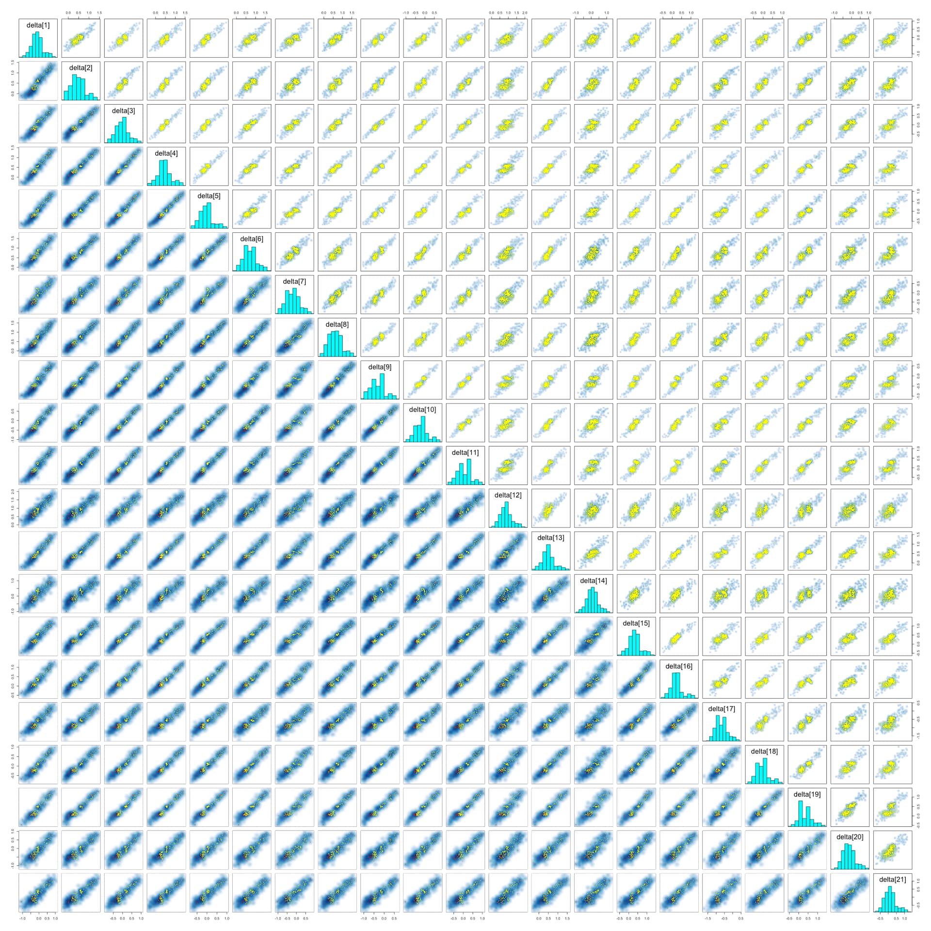
However, I get \hat{R} values greater than 3 for some parameters, including all elements of omega, the standard deviation hyperparameter for s. (This was especially true before I boosted adapt_delta to 0.99.) I know that JAGS uses the relatively unreliable Gibbs sampler, but isn’t that supposed to be for underreporting divergences? I get relatively few divergences now but high rhat, low ESS, and warnings about BFMI.

0.0761141 per iter (2025-07-27 06:10:24.33535)
# A tibble: 15,611 × 10
   variable      mean  median    sd   mad      q5   q95  rhat ess_bulk ess_tail
   <chr>        <dbl>   <dbl> <dbl> <dbl>   <dbl> <dbl> <dbl>    <dbl>    <dbl>
 1 alpha[2,3] -0.510  -0.550  0.510 0.380 -1.31   0.503  3.11     4.55     11.6
 2 alpha[3,4]  0.819   0.795  0.405 0.302  0.193  1.66   3.08     4.55     11.2
 3 alpha[2,4]  1.04    0.949  0.519 0.447  0.240  2.08   3.07     4.56     11.2
 4 delta[4]    0.460   0.457  0.341 0.255 -0.0840 1.14   3.06     4.56     11.4
 5 delta[5]   -0.0281 -0.0408 0.337 0.248 -0.552  0.678  3.05     4.56     11.5
 6 alpha[3,3] -0.405  -0.468  0.406 0.335 -1.04   0.421  3.05     4.56     11.5
 7 delta[11]   0.0588  0.0332 0.368 0.378 -0.530  0.722  3.03     4.57     10.9
 8 delta[8]    0.612   0.595  0.357 0.345  0.0568 1.31   3.00     4.58     11.3
 9 delta[9]   -0.308  -0.344  0.358 0.348 -0.880  0.367  2.99     4.59     11.0
10 delta[10]  -0.190  -0.181  0.351 0.305 -0.733  0.509  2.97     4.59     11.0
# ℹ 15,601 more rows
# ℹ Use `print(n = ...)` to see more rows
Warning messages:
1: There were 57 divergent transitions after warmup. See
https://mc-stan.org/misc/warnings.html#divergent-transitions-after-warmup
to find out why this is a problem and how to eliminate them. 
2: There were 1046 transitions after warmup that exceeded the maximum treedepth. Increase max_treedepth above 10. See
https://mc-stan.org/misc/warnings.html#maximum-treedepth-exceeded 
3: There were 4 chains where the estimated Bayesian Fraction of Missing Information was low. See
https://mc-stan.org/misc/warnings.html#bfmi-low 
4: Examine the pairs() plot to diagnose sampling problems
 
5: The largest R-hat is 3.1, indicating chains have not mixed.
Running the chains for more iterations may help. See
https://mc-stan.org/misc/warnings.html#r-hat 
6: Bulk Effective Samples Size (ESS) is too low, indicating posterior means and medians may be unreliable.
Running the chains for more iterations may help. See
https://mc-stan.org/misc/warnings.html#bulk-ess 
7: Tail Effective Samples Size (ESS) is too low, indicating posterior variances and tail quantiles may be unreliable.
Running the chains for more iterations may help. See
https://mc-stan.org/misc/warnings.html#tail-ess 

Some pairs plots:

alpha

beta

delta

omega

R driver code:

rm(list = ls())

# Replicate the first experiment from the Bullock, Imai, and Shapiro paper
# but using Stan instead of JAGS

library(endorse)
library(dplyr)
library(rstan)
library(posterior)

df <- pakistan

stopifnot(nrow(df) == 5212)

seed <- 1
set.seed(seed)

# a: control
# b: militant groups in Kashmir
# c: militant groups in Afghanistan
# d: Al-Qaeda
# e: Firqavarana Tanzeems
groups <- c("a", "b", "c", "d", "e")

qs <- c("Polio", "FCR", "Durand", "Curriculum")

endorser <- list()
for (q in qs) {
    cols <- sapply(groups, \(g) paste0(q, ".", g))
    df[[q]] <- do.call(coalesce, df[, cols])
    stopifnot(!anyNA(df[[q]]))
 
    endorser[[q]] <- as.matrix(!is.na(df[, cols])) %*% (0:4)
    stopifnot(!anyNA(endorser[[q]]))
}
endorser <- data.frame(endorser)

# division -> province
province <- c(rep.int(1, 8), rep.int(2, 5), rep.int(3, 7), rep.int(4, 6))

# Recode the divisions so that there aren't any missing divisions
bij <- sort(unique(df$division)) # new to old bijection
bij_inv <- match(1:26, bij)      # old to new

data <- list(
    N = nrow(df), J = length(qs), K = length(groups) - 1, D = length(bij), P = 4, L = 5,
    Y = df[, qs],
    T = endorser,
    division = bij_inv[df$division],
    province = province[bij]
)

param_counts <- with(data, 
    list(
        x = N, delta = D, s_treated = sum(endorser > 0), lambda = K * D, 
        omega = K, mu = P, sigma = P, theta = K * P,
        alpha = J * (L - 1), beta = J, phi = K * P)) |> 
    data.frame(row.names = "param_counts") %>%
    mutate(total = sum(.))

print(param_counts)

model <- stan_model("pakistan.stan", model_name = "pakistan1")

print("Starting:")
start_time <- Sys.time()
print(start_time)

iter <- 1000
warmup <- 500
fit_ <- sampling(model,
    iter = iter,
    warmup = warmup,
    data = data,
    seed = seed,
    init = 0,
    chains = 4,
    cores = 8,
    sample_file = "samples",
    diagnostic_file = "diagnostic",
    refresh = 10,
    control = list(adapt_delta = 0.99)
)

end_time <- Sys.time()

elapsed <- difftime(end_time, start_time, units = "mins")[[1]]
cat(sprintf("%.7f per iter (%s)\n", elapsed / iter, toString(end_time)))

ext <- extract(fit_, permuted = FALSE)
summary_ <- summarize_draws(ext)

print(summary_[order(summary_$rhat, decreasing = TRUE), ])

delta_summ <- summary_[startsWith(summary_$variable, "delta"), ]
delta_count <- sapply(1:data$D, \(d) sum(df$division == d))
plot(delta_count, delta_summ$rhat) # or $ess_bulk or $ess_tail

save.image(file = paste0("pakistan.r (", end_time, ").Rdata"))

Thank you for any responses!

1 Like

Kudos for providing a clear question with code, summary results, and figure – makes it a lot easier to understand.

From a cursory glance, a few things stand out as potential issues.

  1. Do you have a strong motivation for placing uniform [0,10] priors on omega, sigma, and phi? Those hard constraints on the parameters like that can be computationally tricky, especially on scale parameters, so I would consider placing a softer constraint on those, a half normal with sd 3 or something.
  2. Your pair plots for alpha and delta suggest a degeneracy in your model. It is constrained somewhat by the prior, but it doesn’t appear to be very favorable structure. This sort of degeneracy in alpha in particular is common in ordinal models like this where you can get identical inferences by shifting all the alphas by some constant in one direction and doing the opposite to eta (and since eta depends on x_i which depends on delta, this degeneracy is likely linked). You can improve this by strengthening the prior constraints on alpha via fixing one of the values or using the new sum_to_zero_vector type.

I would attempt to make those changes and see if that resolves some of the issues you’re seeing.

1 Like

Thank you! I have removed the upper constraint from omega, sigma, and phi and put a normal prior on them. I didn’t truncate the prior like omega ~ normal(0, 3) T [0, ];, but I think this is fine since I kept the lower=0 constraint for all in the parameters block.

I had already tried something similar using a Cauchy prior instead of a Gaussian, but abandoned it since it only got the highest value of \hat{R} down to two point something. (The \text{Uniform}(0, 10) prior comes from the paper and the JAGS file; I wanted to be as true to the original implementation as possible at first.) Here are the 10 highest rhat values (when using only the Gaussian prior):

   variable      mean   median      sd     mad       q5      q95  rhat ess_bulk
    <chr>        <dbl>    <dbl>   <dbl>   <dbl>    <dbl>    <dbl> <dbl>    <dbl>
  1 omega[1]   8.85e-2  7.90e-2 3.65e-2 3.95e-2  4.73e-2  1.56e-1  2.89     4.69
  2 omega[4]   7.79e-2  7.82e-2 3.62e-2 4.52e-2  3.39e-2  1.46e-1  2.70     4.73
  3 omega[2]   6.26e-2  5.39e-2 3.94e-2 4.07e-2  2.12e-2  1.24e-1  2.67     4.78
  4 lp__      -3.89e+3 -4.05e+3 2.27e+3 3.06e+3 -7.44e+3 -6.97e+2  2.61     4.78
  5 omega[3]   1.10e-1  1.24e-1 4.98e-2 5.52e-2  3.88e-2  1.80e-1  2.36     5.05
  6 delta[4]   4.82e-1  4.37e-1 4.17e-1 4.15e-1 -1.07e-1  1.27e+0  2.29     5.09
  7 alpha[2,… -1.64e+0 -1.74e+0 6.25e-1 5.86e-1 -2.53e+0 -5.02e-1  2.27     5.11
  8 alpha[2,… -3.99e-1 -4.86e-1 6.30e-1 5.94e-1 -1.28e+0  7.21e-1  2.27     5.12
  9 alpha[3,… -3.19e-1 -3.71e-1 4.88e-1 4.70e-1 -1.00e+0  5.81e-1  2.26     5.13
 10 alpha[3,…  9.00e-1  8.32e-1 4.85e-1 4.71e-1  2.28e-1  1.81e+0  2.25     5.13

Now the omegas are extremely unstable. This has at least fixed most of the max-treedepth warnings.

Second, when you say “strengthening the prior constraints on alpha via fixing one of the values,” does that mean constraining alpha[:, 1] to zero? I just tried that (keeping the Gaussian priors you suggested) with both a soft constraint and a reparametrization (so alpha becomes array[J] positive_ordered[L - 2]).
With the soft constraint, the convergence is a bit better, but the rhat for omega and lambda are still > 2, and the tree-depth warnings are back.

# A tibble: 15,611 × 10
   variable    mean median     sd     mad      q5    q95  rhat ess_bulk ess_tail
   <chr>      <dbl>  <dbl>  <dbl>   <dbl>   <dbl>  <dbl> <dbl>    <dbl>    <dbl>
 1 omega[4]  0.0457 0.0431 0.0132 0.0153   0.0273 0.0684  2.62     4.80     16.9
 2 lambda[4… 0.0984 0.105  0.0434 0.0432   0.0190 0.155   2.44     4.92     12.0
 3 lambda[3… 0.0881 0.0928 0.0752 0.0682  -0.0456 0.215   2.43     4.96     15.1
 4 lambda[1… 0.129  0.114  0.0623 0.0678   0.0470 0.247   2.39     4.98     12.1
 5 lambda[3… 0.0265 0.0220 0.0509 0.0589  -0.0532 0.109   2.38     4.98     13.9
 6 lambda[3… 0.152  0.145  0.0459 0.0543   0.0913 0.230   2.31     5.09     16.7
 7 lambda[2… 0.0674 0.0867 0.0642 0.0581  -0.0592 0.141   2.29     5.06     14.5
 8 lambda[2… 0.0572 0.0662 0.0480 0.0551  -0.0258 0.125   2.28     5.11     11.2
 9 omega[2]  0.0456 0.0455 0.0113 0.00753  0.0224 0.0650  2.20     5.17     16.4
10 lambda[3… 0.0709 0.0656 0.0362 0.0458   0.0167 0.129   2.19     5.19     31.3

The alpha plots look more blobby, which is good. However, this is mostly because of the constraint placed on alpha[:, 1] (most of the blobs are in the upper five rows and leftmost five columns).


However, beta has become auto-correlated.


Note that the pairs plot for omega no longer has distinct lines parallel to the axes.

The forums only let me upload four images, so here is a zip file containing all pairs plots for three experiments: your first suggestion only, your first suggestion with a soft constraint on alpha, and your first suggestion with a hard constraint/reparametrization of alpha.

With the hard constraint, the rhat values have increased again!

# A tibble: 15,607 × 10
   variable       mean   median      sd     mad       q5      q95  rhat ess_bulk
   <chr>         <dbl>    <dbl>   <dbl>   <dbl>    <dbl>    <dbl> <dbl>    <dbl>
 1 omega[2]    6.40e-2  5.67e-2 3.66e-2 3.29e-2  2.45e-2    0.150  3.42     4.47
 2 omega[4]    7.73e-2  5.25e-2 6.32e-2 4.01e-2  1.47e-2    0.195  3.41     4.47
 3 omega[1]    6.95e-2  6.95e-2 2.79e-2 3.10e-2  2.73e-2    0.115  2.81     4.71
 4 omega[3]    1.08e-1  6.08e-2 8.32e-2 5.35e-2  2.38e-2    0.244  2.70     4.75
 5 lp__       -4.20e+3 -4.46e+3 1.84e+3 1.93e+3 -6.49e+3 -559.     2.41     4.96
 6 lambda[3,…  1.35e-1  2.03e-1 2.32e-1 1.67e-1 -2.73e-1    0.457  2.34     5.00
 7 lambda[1,… -5.04e-2 -2.61e-2 1.49e-1 1.35e-1 -3.36e-1    0.146  2.12     5.30
 8 lambda[3,…  2.67e-1  2.59e-1 1.32e-1 1.39e-1  8.06e-2    0.534  2.01     5.50
 9 lambda[4,…  1.26e-1  1.20e-1 9.09e-2 8.60e-2  7.84e-3    0.278  2.01     5.56
10 lambda[3,…  5.97e-2  6.90e-2 1.65e-1 1.78e-1 -1.96e-1    0.345  1.95     5.55

Strong correlation remains within each alpha[j]. Should I just try cranking up max_treedepth to 14? Or is this too characteristic of a degenerate model?

Yes, when you have a parameter constraint like lower=0, you don’t need to put any distribution truncation.

Two more thoughts:

  1. The \beta values are now exhibiting the linear degeneracy from before. To clarify what I think is going on here, your ordered probit model is:
Y[i, j] ~ ordered_probit(eta, alpha[j]);

which is ultimately fitting ordered categories by looking at \eta - \alpha_j = \beta_j ( x_i + s) - \alpha_j where E[x_i] = \delta_i and E[s_{ijk} | k > 0] = \lambda_{jk}. So there are a few ways that one can produce identical likelihoods by translating some of these parameters. This is what was seen before with the linear degeneracy in the posteriors of \alpha and \delta. It seems that by implementing some constraints, the degeneracy has shifted a bit to \beta. You can probably resolve this further by placing more constraints (such as fixing one of the \beta components to 1), but you probably want to think a good bit about how these parameters should be interpreted and how the various constraints would change those interpretations.

  1. With seemingly a lot of issues concentrating around the \lambda and \omega parameters, which are pretty hierarchical, I would try shifting your model to use a non-centered parametrization. Especially in instances where you have multiple layers of hierarchy and perhaps not a huge amount of data to constrain the posterior inferences, these sorts of centered parametrizations create very tricky posterior geometries that can cause issues.

I don’t know what your data looks like, but with this sort of structure, you may be running into general issues with the appropriately inform some of these hierarchical parameters. Hierarchical variance parameters like \omega often exhibit issues like this and you may want to try having a single \omega rather than varying by endorser, at least to see if that resolves some of the computational difficulties.

Hierarchical models with many latent parameters like this are often better built by starting with a simpler model and iteratively expanding the model until issues pop up (if only to simplify the model debugging process).

1 Like