I think log(E/PT) is just the log of the MLE of the baseline hazard (assuming a constant baseline hazard, i.e. survival times have exponential law). It’s a good heuristic, I also sometimes use.
@sambrilleman et al., what about posterior predictive checks, i.e. being able to generate (uncensored) survival times? I usually use this in my workflow and found the following algorithm to work well for the M-spline case. It generates conditioned survival times for the “patients” without censoring:

See also this collection of related snippets I created for a recent meetup.
I call this conditioned posterior predictive checks, because posterior samples a generated conditioned to be less equal the length of study (or maximal event time observed). This is because I’ve seen cases where there was rather large support of the survival distribution on times larger then study length. Here unconditioned or standard posterior predictive checks would indicate a bad model, see this intro-level case study on Bayesian Survival Models in Stan, that I wrote, where I show this for a public dataset.
Lastly, what would we do in the case we would like to generate samples from the posterior predictive distribution without the conditioning. I am a bit concerned about the fact that the i-splines all are zero (or undefined?) beyond the right most knot (in time). One option would be to pick the right most knot large enough in advance (meaning larger than the observed samples), but this workaround seems suboptimal to me.
This is exactly the rationale. You can either think of it as the MLE assuming an exponential distribution or just a simple naive estimator to get a rescaling factor. Truthfully, I even use MLEs for centering prior distributions on the Weibull scale and shape parameters – it’s just more data “double dipping” than I would suggest as a default strategy.
I wish I had seen this earlier. I just spent this afternoon implementing a posterior predictive checks based on Kaplan-Meier survival estimates and it looks like you’ve already done that.
Isn’t this just generating from a truncated event time distribution where the truncation takes the form of an upper bound? Is that what you mean by conditioned: you are conditioning on getting to observe the event, so you are forcing it to be less than T^*?
Yes. I do this by rejection sampling, essentially. I’ve had some people suggesting to me to take the minimum of the generated sample and the maximum of observed event times, but this doesn’t seem to be right…
Here is some snippet:
generated quantities {
    vector[N_uncensored] times_uncensored_sampled;
    {
        real tmp;
        real max_time;
        real max_time_censored;
        max_time = max(times_uncensored);
        max_time_censored = max(times_censored);
        if(max_time_censored > max_time) max_time = max_time_censored;

        for(i in 1:N_uncensored) {
            tmp= max_time + 1;
            while(tmp > max_time) {
                tmp = exponential_rng(exp(intercept+X_uncensored[i,]*betas));
            }
            times_uncensored_sampled[i] = tmp;
        }
    }

}
I thought I was missing something because it was hard to invert due to the splines, but maybe not since you are using exponential_rng in your example code. To draw an exponential random number with an upper bound ub without rejection sampling, you could use the following (untested) code:
real exponential_ub_rng(real beta, real ub) {
    real p = exponential_cdf(ub, beta);  // cdf for bounds
    real u = uniform_rng(0, p);
    return (-log1m(u) / beta);  // inverse cdf for value
  }
The beta here matches the Stan manual parameterization and would be exp(intercept+X_uncensored[i,]*betas) in your notation.
This is somewhat tangential, though. You are presupposing that the same individuals will be censored (or not censored) in any replicated data, and I don’t see why that would be the case. Is it possible that when people are suggesting you take the minimum, they mean to suggest you apply artificial censoring at T^*? That is what I do. However, it requires knowing a potential censoring time for each individual. For example, if the study ends on Dec 31 and I know they entered the study on June 3, I know exactly when they would have been censored, even if I observe the event to occur in August (and thus do not directly observe the censoring “event” time). Alternately, you may know that everyone will be followed up for a maximum of 90 days. For some censoring mechanisms, this knowledge is not possible, unfortunately.
Thanks, this useful!
Your sedond comment is applicable when there is no drop out, right? Otherwise what do you think about the approach to have another event model, that is conditionally independent of the first one, given covariates. One would then use this to describe the censoring / dropout process (inverting event status indicators). In the generative posterior predictive sampling step, one could then use the minimum of the two event times generated, and cap this by the max study length…
Yes, I am thinking of administrative censoring, which is the form that my data set has and the easiest to justify as being a noninformative censoring mechanism. Everyone is censored at 90 days if they are still alive to be censored. Maybe a better way of thinking about this distinction is not as non-informative vs. informative as I’ve been doing, but fixed vs. random.
All of the posterior predictive options I’ve seen have required some amount of outside information about censoring. I have the easy case where the censoring time C_i = 90 \ \forall \ i, but colleagues have also worked with random study entry time, which results in known – if individual-specific – values of C_i regardless of whether censoring is observed to occur. (I will ask my colleagues if there is a draft they could put on arXiv.)
If I’m understanding you correctly, your goal is to develop a posterior predictive approach for noninformative but random censoring? That would certainly enhance the usefulness of posterior predictive checks for survival data. Building a model for the censoring process would be a good start, but I’m not sure how you could deal with the fact that you know your event time model shouldn’t be trusted beyond T^*. It would be annoying to discover your model fit is “bad” because of predictions you never intended to take seriously anyway. Perhaps that is a justification for building a dropout/“early censoring” model and enforcing an administrative censoring event at T^* in your replicate data sets. You’d need to make sure any summary measures calculated from the posterior predictions account for censoring.
Excuse my ignorance, but my understanding was that B-spline basis terms sum to 1. But is it also true that the coefficients on the M-splines must sum to 1? I didn’t realise that. If so, the simplex declaration definitely makes sense. But does this constraint also hold true if the user specifies B-splines on the log baseline hazard?
But if we have a simplex declaration for the spline coefficients, with a Dirichlet prior, it might cause some confusion with the priors specified in the stan_surv call. At the moment the prior_aux argument refers to the spline coefficients when basehaz is set to M-splines or B-splines, and refers to the shape parameter when basehaz is Weibull or Gompertz. Of course, for the latter, the Dirichlet prior makes no sense, so it is not clear what we would make the default value for prior_aux since the available choices of prior depend on the chosen type of parametric model.
Any thoughts?
Yeah this prior sounds like a good idea for the intercept. In stan_jm I basically use something equivalent in which I subtract the log of the crude event rate, i.e. log(E / PT), from the linear predictor, rather than centring the prior on it. It is mathematically equivalent of course, but just means that the user can still define their prior_intercept as being centred on zero which is a bit more intuitive I think if, say, they just want to change the prior distribution to cauchy or something (and avoids us messing with their choice of prior internally, aside from the autoscaling).
I think centring the intercept (or equivalently, the prior on the intercept) around the crude event rate is probably reasonable and justified for the same reasons rstanarm uses the autoscaling. But going as far as centering the shape parameter would definitely start feeling too much like a double use of the data I think. Although it’s not exactly clear where to draw the line! But I think the prior on the shape parameter is far less likely to be problematic compared with the prior on the intercept (famous last words).
This seems really cool. In the examples you linked to, the predicted survival times appear more positively skewed than the observed event times, even with the conditioning – is this just because of the model fit? Or is it something related to the approach?
Should we even be allowing “unconditional” predictions (i.e. beyond the final event time)? Wouldn’t those simulated event times be drawn from a part of the survival time distribution for which we have no observed data (i.e. we don’t know how the cumulative hazard behaves in that region, yet we are taking it’s estimated value and inverting it), and hence that type of extrapolation seems kinda dangerous? Not to mention the quality of those predictions couldn’t be assessed directly against any observed data anyway?
I once felt that way. I became less principled when I wanted to run a simulation study and everything kept blowing up due to outrageous values for the shape parameter. It is particularly bothersome when specifying multiple hazard models like I have in my application. I agree it feels too much like double dipping for general use, but do not discount the ability of a bad Weibull shape value to totally wreck your model. Shape parameters can be finicky! For me I know I have crossed my personal line because I have to use an iterative procedure to obtain the MLE. If it is a simple rescaling by a formula I can write out like the \log(E/PT), I am okay with it. But if Step 1 of my Bayesian procedure is to verify that my frequentist estimation procedure converged, I feel I am firmly in “double dip” territory.
W.l.o.g. assume the covariate vector (per individual) has dimension 1, then we have for the cumulative hazard at time t for an individual with covariate x the following expression
H(t;x;\gamma) = e^{\beta_0 + \beta_1 x}\sum_{k=1}^{m} \gamma_k I_k(t)
Now, suppose the spline coefficients do not sum to 1 and denote by 1\neq s=\sum_{k=1}^m \gamma_m the sum of spline coefficients. Then we can define normalised spline coefficients \tilde{\gamma}_k \equiv \gamma_k / s and obtain
H(t;x;\tilde{\gamma}) = e^{\beta_0+\log(s) + \beta_1 x}\sum_{k=1}^{m} \tilde{\gamma}_k I_k(t)
Thus we have an identifiably problem for \beta_0 and \log(s), if we keep the intercept \beta_0 in our model. So either we leave the intercept out and use un-normalised spline coefficients or we keep the intercept and use normalised spline coefficients. This is true if we use B- or M- splines on the baseline hazard.
When we use B- or M-splines on the log-hazard scale (think Royston & Parmar), the above argument does not apply (so there is no apparent identifiability problem for the intercept).
What about we use a logit or probit transformation to get from raw coefficients to simplex coefficients. The (unconstrained) normal priors currently used as default in stan_surv, would then be for the raw coefficients (see Ch 22.2., Unconstrained Priors: Probit and Logit in the Stan Manual 2.17.)
To be honest, I do not know. I haven’t made up my mind about how to improve this / what the cause is.
Good point, but what would you do in cases where you need to “extrapolate” in an ongoing study using the survival model (potentially in a decision making framework; e.g. adjustments of treatments)? That is you are right into a study (where you haven’t observed many events yet, and have thus mostly censoring) and would like to predict survival times of patients.
Regarding default prior choices for the intercept, I think we should not spend too much time thinking about good default priors, but we should rather encourage (and support) users to do prior predictive checks to find problem specific appropriate priors.
@ermeel @lcomm Hey guys, just to update… today I had a go at making the following changes to stan_surv:
- I centered the predictor matrix.
- I centered the baseline hazard around the crude event rate (i.e. \log(E/PT)).
- I removed the intercept (
intercept = TRUE) from the spline basis whenbasehaz = "ms"orbasehaz = "bs"and included an intercept parameter in the linear predictor instead. - I extended upon 3. to deal with the identifiability issue when
basehaz = "ms"by taking the raw M-spline coefficients defined on the positive real line, and transforming them to a simplex using Stan’ssoftmaxfunction.
Steps 1. and 2. seemed to work fine. The result is that the prior for prior_intercept (for exponential, Weibull and Gompertz) or prior_aux (for M-spline and B-spline) corresponds to the (log) baseline hazard when centered around the (log) crude event rate and at the mean values of each of the covariates. I then decided to back-transform the intercept (for exponential, Weibull and Gompertz) or spline coefficients (for M-spline and B-spline) in the generated quantities block before they are returned to the user, so that the centering adjustments aren’t required when making posterior predictions. You can see these changes on this comparison view (in particular, the generated quantities block in the surv.stan file).
However, Steps 3. and 4. seemed to cause problems with the M-spline baseline hazard. Removing the intercept from the spline basis and including an explicit intercept in the linear predictor seems to have a detrimental effect on the sampling. Fitting a simple model to a simulated dataset with one binary covariate and a Weibull baseline hazard, I found that the constrained (simplex) spline coefficients led to sampling times that were about 20 times longer than when I used the unconstrained spline coefficients (with the intercept included in the spline basis). It may be something to do with priors, but I have tried a variety of scale parameters for prior_intercept and/or prior_aux and couldn’t seem to improve things. The model does return the correct parameter estimates (i.e. the estimated hazard ratio is similar to the value used in the simulation model) and baseline hazard (checked informally using the ps_check function), but sampling is very slow. If you want to see how I implemented the constrained spline coefficients, then I have pushed those changes on this branch – but specifically you might want to check out the comparison view that shows how I now generate the constrained spline coefficients.
Because of the difficulties sampling I’m tempted to just keep the intercept absorbed into the spline basis. The model just seems to perform better, but I can’t pin down why. I think this must have been the behaviour that led me to adopt the intercept = TRUE approach in the first place. But, I’m perfectly happy to adopt the other approach if we can get it to work. Since, I do agree, that it is a bit more intuitive for the user to have prior_intercept be relevant for all types of baseline hazard.
Just another follow on from this. I did a bit more digging today and it turns out the M-spline model samples fine when using the constrained spline coefficients with a uniform prior over the simplex, as originally proposed by @ermeel.
The sampling difficulties I mentioned yesterday are only encountered when trying to define a prior (e.g. normal, Cauchy, t) on the raw unconstrained spline coefficients, and then transforming them to the constrained space (i.e. a unit simplex) using the softmax function.
So… if we opt for an explicit intercept parameter for all types of baseline hazard that will be ok. But the question that remains is what to make the default prior for prior_aux. Perhaps the best option is to have the default value for prior_aux so-called “missing” in the function signature, e.g.
stan_surv(formula, data, basehaz = "ms", basehaz_ops, qnodes = 15,
  prior = normal(), prior_intercept = normal(), prior_aux,
  prior_smooth = exponential(autoscale = FALSE), prior_PD = FALSE,
  algorithm = c("sampling", "meanfield", "fullrank"),
  adapt_delta = 0.95, ...)
and just describe the default value in the documentation, something like…
prior_aux: The prior distribution for “auxiliary” parameters related to the baseline hazard. The relevant parameters differ depending on the type of baseline hazard specified in the basehaz argument. The following applies (however, for further technical details, refer to the stan_surv: Survival (Time-to-Event) Models vignette):
basehaz = "ms": the auxiliary parameters are the coefficients for the M-spline basis terms on the baseline hazard. These coefficients are defined using a simplex; that is, they are all between 0 and 1, and constrained to sum to 1. This constraint is necessary for identifiability of the intercept in the linear predictor. The default prior is a Dirichlet distribution with a scalar concentration parameter set equal to 1. That is, a uniform prior over all points defined within the support of the simplex. Specifying a scalar concentration parameter > 1 supports a more even distribution (i.e. a smoother spline function), while specifying a scalar concentration parameter < 1 supports a more sparse distribution (i.e. a less smooth spline function).basehaz = "bs": the auxiliary parameters are the coefficients for the B-spline basis terms on the log baseline hazard. These parameters are unbounded. The default is a normal distribution with mean 0 and scale 20.basehaz = "exp": there is no auxiliary parameter, since the log scale parameter for the exponential distribution is incorporated as an intercept in the linear predictor.basehaz = "weibull": the auxiliary parameter is the Weibull shape parameter, while the log scale parameter for the Weibull distribution is incorporated as an intercept in the linear predictor. The auxiliary parameter has a lower bound at zero. The default is a half-normal distribution with mean 0 and scale 2.basehaz = "gompertz": the auxiliary parameter is the Gompertz scale parameter, while the log shape parameter for the Gompertz distribution is incorporated as an intercept in the linear predictor. The auxiliary parameter has a lower bound at zero. The default is a half-normal distribution with mean 0 and scale 2.Currently,
prior_auxcan be a call to dirichlet, normal, student_t, cauchy, or exponential. Seepriorsfor details on these functions. Note that not all prior distributions are allowed with all types of baseline hazard. To omit a prior —i.e., to use a flat (improper) uniform prior— setprior_auxtoNULL.
Maybe @bgoodri also has some advice on this.
@sambrilleman, I think the documentation for prior_aux is fine. I propose we stick with it and see how it is received by users and in case it causes too much confusion, we change it.
That seems fine, but I would do prior_aux = dirichlet() in the signature. We already have that in rstanarm for variance components.
Fyi, I’ve just merged AFT models into the survival branch. Covariate effects can be incorporated using time-fixed or time-varying acceleration factors. Although, at the moment only an exponential or Weibull can be specified for the baseline survival distribution. I’ve added a bunch of details on the model formulations to the vignette.
The difficulty with doing this is that if the user changes the baseline hazard from the default setting (which they are quite likely to do), for example, they specify basehaz = "weibull", then the Dirichlet prior isn’t valid and they will get an error. So it is a bit of pain. Every time they change the baseline hazard they would have to change prior_aux too.
I’ve actually been playing around with the M-spline model more, based on the simplex and Dirichlet prior for the M-spline coefficients. But it does something that surprises (worries?) me… Increasing the number of knots in the M-spline function for the baseline hazard doesn’t necessarily increase the flexibility of the curve. For example, say I increase the number of knots from 5 to 50, I would expect the curve to be much more “wiggly”. Instead, it isn’t. In the examples I ran, the Dirichlet prior forces most of the coefficients to zero. In other words, the Dirichlet prior seems to enforce smoothing. Is this expected? If so, that seems ok. But I didn’t realise that the Dirichlet would act as a smoothing prior.
That is an interesting observation! I do not have an explanation for this, but maybe one can understand this by considering how “probability-mass” is distributed in high-dimensional simplexes through the Dirichlet, maybe @betanalpha has an intuition here?
Regarding the expected “wiggliness”: This might also be less severe for this particular case, since we have M-splines here that are non-negative and are also combined using non-negative weights. I would expect (this is a very vague intuition) that the “wiggliness” is therefore suppressed, since we cannot have cancellation effects of splines and coefficients…
Out of curiosity, did you find different choices of priors for the m-/i-spline coefficients that can lead to a very “wiggly” curve, as the number of knots is increased?
The behavior of the Dirichlet distribution as the dimensionality increases depends on the configuration of the hyperparameters. Let’s assume that they’re all set to the same value, \alpha. For \alpha \le 1 then as the dimensionality increases the Dirichlet will concentrate around the corners where most of the values hover around zero. For \alpha > 1 there will be a soft concentration in the center of the simplex.
Thanks!
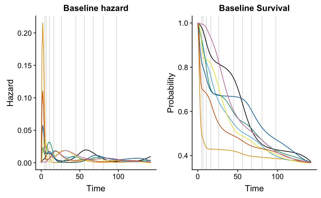
Here are some examples with 13 knots and different values of \alpha. The figures show prior samples of the baseline hazard curve and induced baseline survival curves, that is
h(t) = e^{\beta_0} \sum_{k=1}^{m} \gamma_k M_k(t)
and
S(t) = \exp\left(-e^{\beta_0} \sum_{k=1}^{m} \gamma_k I_k(t)
\right)
where the gammas have a joint Dirichlet prior with common \alpha parameter and \beta_0 has a Normal(-5,2) prior. The M_k,I_k are, respectively, the corresponding m-/i-spline basis functions at time point t. Each of the figures shows 8 samples.
\alpha=1:

\alpha=2:

\alpha=4:

\alpha=8:

\alpha=0.5
\alpha=0.25:

\alpha=0.125

I guess what it is happening for low values of \alpha, we effectively see a randomly chosen basis function here, where as for large values of \alpha we see, roughly, an average basis function…
To quote Wikipedia:
A concentration parameter of 1 (or k , the dimension of the Dirichlet distribution, by the definition used in the topic modelling literature) results in all sets of probabilities being equally likely, i.e. in this case the Dirichlet distribution of dimension k is equivalent to a uniform distribution over a k-1 -dimensional simplex. Note that this is not the same as what happens when the concentration parameter tends towards infinity. In the former case, all resulting distributions are equally likely (the distribution over distributions is uniform). In the latter case, only near-uniform distributions are likely (the distribution over distributions is highly peaked around the uniform distribution). Meanwhile, in the limit as the concentration parameter tends towards zero, only distributions with nearly all mass concentrated on one of their components are likely (the distribution over distributions is highly peaked around the k possible Dirac delta distributions centered on one of the components, or in terms of the k -dimensional simplex, is highly peaked at corners of the simplex).
Let’s say you have a \mathrm{Dirichlet}(\alpha_1, \dots, \alpha_k) prior. According to this paper, the effective sample size of that prior information is \sum_i^{k} \alpha_i. So if you keep \alpha_1 = \alpha_2 = \dots = \alpha_k constant as you increase k you are effectively asserting a stronger a priori belief that the basis weights are equal. Is that desirable?