Subject-specific vs population-averaged effects in brms longitudinal bernoulli regression model

llewmills · May 22, 2020, 12:06am

I am analysing an experiment looking at abstinence rates among participants in a clinical drug and alcohol trial. There were two groups, those who received the new treatment and those who received placebo. Abstinence during the previous week was measured at 0 (baseline), 4, 8, 12, and 24 weeks. There was a high rate of attrition/missing data so that of the 128 that commenced the trial, only 55 supplied data at follow-up. I want to estimate the group difference in odds of abstinence at each time point, controlling for the other time points. I am especially interested in the difference in odds of abstinence at week 24 (controlling for all the other timepoints).

Here is the data.

df <- data.frame(id = factor(rep(1:128,each=5)),
                 time = factor(rep(c(0,4,8,12,24),times=128)),
                 group = factor(c(rep("placebo",335),rep("treatment",305))),
                 abs = c(0, 0, 0, 0, 0, 0, NA, NA, NA, NA, 0, NA, NA, NA, NA, 0, 1, 1, NA, 1, 0, 0, 0, NA, NA, 0, 0, 1, NA, 0, 0, 0, NA, NA, 1, 0, NA, NA, NA, 0, 0, 0, NA, NA, NA, 0, NA, NA, NA, 1, 0, 0, NA, NA, NA, 0, 0, 0, 0, 0, 0, 0, 0, 0, 0, 0, 0, NA, NA, NA, 0, NA, NA, NA, NA, 0, 0, 0, 0, 0, 0, 0, 0, 0, 0, 0, 0, NA, NA, 0, 0, NA, NA, NA, NA, 0, 0, 0, 0, 0, 0, 0, 0, 0, NA, 0, 0, 0, 0, NA, 0, NA, NA, NA, NA, 0, 0, NA, NA, NA, 0, 0, NA, 0, 0, 0, 0, 0, 0, NA, 0, 0, 0, 0, 0, 0, 0, 0, 0, NA, 0, 0, NA, NA, NA, 0, 0, 0, 0, 0, 0, 0, 0, 0, NA, 0, 0, NA, 0, 0, 0, 0, 0, NA, 0, 0, 0, 0, 0, NA, 0, 0, 0, 0, 0, 0, 0, 0, 0, NA, 0, NA, NA, NA, NA, 0, 0, 0, NA, NA, 0, 1, 1, 1, NA, 0, 0, 0, 0, NA, 0, 0, 0, NA, NA, 0, 0, 0, 0, NA, 0, 0, 0, 0, 0, 0, NA, NA, NA, NA, 0, 0, NA, NA, NA, 0, 0, 1, 1, NA, 0, 1, 1, 1, 0, 0, 0, 0, 0, 0, 0, 1, 1, 1, 0, 0, 0, 0, 0, NA, 0, 0, 1, 1, 1, 0, 0, 0, NA, NA, 0, 0, 0, 0, NA, 0, 0, 0, 0, 1, 0, 0, 1, 1, 0, 0, 0, 0, 0, 0, 0, 1, 0, 0, NA, 0, 0, NA, NA, NA, 0, 0, 0, 0, 0, 0, NA, NA, NA, NA, 0, 1, 1, 1, 1, 0, 0, 0, 0, 0, 0, 0, NA, NA, NA, 0, NA, NA, NA, NA, 0, 0, 0, 0, NA, 0, 0, 0, 0, NA, 0, NA, NA, NA, NA, 0, 0, 0, 0, 1, 0, 1, NA, NA, 0, 0, 0, 0, NA, 0, 0, 0, 0, 0, 0, 0, 0, 0, NA, NA, 0, NA, NA, NA, NA, 0, NA, NA, NA, NA, 0, NA, NA, NA, NA, 0, 0, 0, 0, 1, 0, 0, 1, 0, 1, 0, 0, 0, 0, 0, 0, 0, NA, 0, NA, 0, NA, NA, NA, NA, 0, 0, 0, 0, 0, 0, 0, NA, NA, NA, 0, 0, NA, 0, NA, 0, NA, 1, NA, 1, 0, 0, NA, NA, NA, 0, 1, 1, 1, 1, 0, 0, 0, NA, NA, 0, NA, NA, NA, NA, 0, NA, NA, NA, NA, 0, 0, 0, 0, NA, 0, 0, 0, 0, NA, 0, 0, NA, 0, NA, 0, 0, 0, 0, 0, 0, NA, NA, NA, NA, 0, 0, 0, 0, 0, 0, 0, 1, 1, 0, 0, NA, NA, NA, NA, 0, 0, NA, NA, NA, 0, 0, 0, 0, NA, 0, 0, NA, 0, NA, 0, 0, 0, 0, NA, 0, 0, 0, 0, NA, 0, 0, 0, 0, NA, 0, NA, NA, NA, NA, 0, 1, 1, 1, 1, 0, NA, NA, NA, NA, 0, 0, NA, NA, NA, 0, 0, 1, 1, 1, 0, 1, 1, 1, 1, 0, 1, 1, 1, 1, 0, 1, 1, 1, 1, 0, 0, 0, 1, 0, 0, 0, 0, 1, 1, 0, 0, 0, 0, 0, 0, 0, NA, NA, NA, 0, NA, NA, NA, NA, 0, 0, 0, 0, 1, 0, 0, NA, NA, NA, 0, 0, 0, 0, 0, 0, 0, NA, NA, NA, 0, 1, 1, 1, 1, 0, 0, 1, 0, NA, 0, 0, 0, 0, 0, 0, 0, 0, 0, 1, 0, 0, NA, 0, NA, 0, 0, NA, 0, NA, 0, 0, 0, 0, NA, 0, 0, NA, NA, NA))

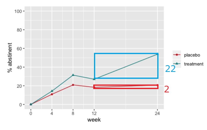
The proportions of the observed cases who were abstinent over time look like this

Rplot04

Which, on face value, looks like a decent treatment effect, especially at week 24.

Here is the model in brms

m <- brm(abs ~ group*time + (1|id),
         data = df,
         family = 'bernoulli',
         prior = set_prior("normal(0,5)"),
         warmup = 1e3,
         iter = 1.1e4,
         chains = 4, 
         cores = 4,
         seed = 1234)

print(m, pars = "b")

# output

# Family: bernoulli 
# Links: mu = logit 
# Formula: abs ~ group * time + (1 | id) 
# Data: df (Number of observations: 440) 
# Samples: 4 chains, each with iter = 11000; warmup = 1000; thin = 1;
# total post-warmup samples = 40000
# 
# Group-Level Effects: 
#   ~id (Number of levels: 128) 
#               Estimate Est.Error l-95% CI u-95% CI Rhat Bulk_ESS Tail_ESS
# sd(Intercept)     4.12      0.84     2.73     6.02 1.00    12899    21612
# 
# Population-Level Effects: 
#                       Estimate Est.Error l-95% CI u-95% CI Rhat Bulk_ESS Tail_ESS
# Intercept               -10.60      1.90   -14.67    -7.24 1.00    16235    21747
# grouptreatment           -0.59      1.94    -4.49     3.13 1.00    19024    24606
# time4                     4.93      1.53     2.17     8.15 1.00    21260    25054
# time8                     6.60      1.57     3.76     9.90 1.00    20332    23917
# time12                    6.35      1.59     3.46     9.69 1.00    21334    25006
# time24                    5.71      1.56     2.85     8.98 1.00    22546    25676
# grouptreatment:time4      1.62      1.95    -2.10     5.53 1.00    21214    27577
# grouptreatment:time8      1.85      1.95    -1.90     5.77 1.00    20731    26607
# grouptreatment:time12     1.88      1.97    -1.89     5.87 1.00    20978    28585
# grouptreatment:time24     4.26      2.04     0.37     8.37 1.00    21738    28906
# 
# Samples were drawn using sampling(NUTS). For each parameter, Eff.Sample 
# is a crude measure of effective sample size, and Rhat is the potential 
# scale reduction factor on split chains (at convergence, Rhat = 1).

Now, this model converges, unlike equivalent frequentist models in geepack, lme4, GLMMadaptive and glmmTMB packages. I assume this is because of the regularising priors helping guide the algorithm which values to spend its time exploring.

The thing that troubles me is the size of the log-odds coefficients for the grouptreatment:time24. Exponentiating 4.26 yields an odds ratio of 70.8! This does not seem like a reliable estimate to me, given that the proportion abstinent at this time point in the placebo group is 6/29 = 20.7% and the proportion in the treatment group is 14/26 = 53.8%

So why are these log-odds coefficients so high?

The output calls them ‘population-level’ effects but is it possible they in fact subject-specific effects of the sort usually returned by these models (see https://stats.stackexchange.com/questions/444380/confused-about-meaning-of-subject-specific-coefficients-in-a-binomial-generalise)?

There is a function in brms called ‘conditional_effects’. Would this provide better estimates of the odds ratio at week 24?

Another possibility that occurred to me is that the estimates at week 24 are unstable because there are so few data at this time point (n=55) compared to week 0 (n=128).

I guess my problem is I don’t run a whole lot of panel models with binary outcomes. Maybe the estimates of the week-24 group effect are fine, but my gut tells me they’re not. I just need some advice from people with more experience with these sorts of models.

Jean_Billie · May 22, 2020, 11:18pm

Because the missing data is a high rate, it seems to me that the analysis reflects the weeks 12 and 24. And if so, then the baseline will be the 12 weeks instead 0 week. Then if we focus only on the weeks 12 and 24, then the high odds ratio seems reasonable.

The valiation of frequency of placebo between week12 and 24 is too small, thus in my view such a small frequency gives the very large odds ratio.

Note that the codes of the data frame has an error. Is it the following?

df <- data.frame(id = factor(rep(1:128,each=5)),
                 time = factor(rep(c(0,4,8,12,24),times=128)),
                 group = factor(c(rep("placebo",335),rep("treatment",305))),
                                abs = c(0, 0, 0, 0, 0, 0, NA, NA, NA, NA, 0, NA, NA, NA, NA, 0, 1, 1, NA, 1, 0, 0, 0, NA, NA, 0, 0, 1, NA, 0, 0, 0, NA, NA, 1, 0, NA, NA, NA, 0, 0, 0, NA, NA, NA, 0, NA, NA, NA, 1, 0, 0, NA, NA, NA, 0, 0, 0, 0, 0, 0, 0, 0, 0, 0, 0, 0, NA, NA, NA, 0, NA, NA, NA, NA, 0, 0, 0, 0, 0, 0, 0, 0, 0, 0, 0, 0, NA, NA, 0, 0, NA, NA, NA, NA, 0, 0, 0, 0, 0, 0, 0, 0, 0, NA, 0, 0, 0, 0, NA, 0, NA, NA, NA, NA, 0, 0, NA, NA, NA, 0, 0, NA, 0, 0, 0, 0, 0, 0, NA, 0, 0, 0, 0, 0, 0, 0, 0, 0, NA, 0, 0, NA, NA, NA, 0, 0, 0, 0, 0, 0, 0, 0, 0, NA, 0, 0, NA, 0, 0, 0, 0, 0, NA, 0, 0, 0, 0, 0, NA, 0, 0, 0, 0, 0, 0, 0, 0, 0, NA, 0, NA, NA, NA, NA, 0, 0, 0, NA, NA, 0, 1, 1, 1, NA, 0, 0, 0, 0, NA, 0, 0, 0, NA, NA, 0, 0, 0, 0, NA, 0, 0, 0, 0, 0, 0, NA, NA, NA, NA, 0, 0, NA, NA, NA, 0, 0, 1, 1, NA, 0, 1, 1, 1, 0, 0, 0, 0, 0, 0, 0, 1, 1, 1, 0, 0, 0, 0, 0, NA, 0, 0, 1, 1, 1, 0, 0, 0, NA, NA, 0, 0, 0, 0, NA, 0, 0, 0, 0, 1, 0, 0, 1, 1, 0, 0, 0, 0, 0, 0, 0, 1, 0, 0, NA, 0, 0, NA, NA, NA, 0, 0, 0, 0, 0, 0, NA, NA, NA, NA, 0, 1, 1, 1, 1, 0, 0, 0, 0, 0, 0, 0, NA, NA, NA, 0, NA, NA, NA, NA, 0, 0, 0, 0, NA, 0, 0, 0, 0, NA, 0, NA, NA, NA, NA, 0, 0, 0, 0, 1, 0, 1, NA, NA, 0, 0, 0, 0, NA, 0, 0, 0, 0, 0, 0, 0, 0, 0, NA, NA, 0, NA, NA, NA, NA, 0, NA, NA, NA, NA, 0, NA, NA, NA, NA, 0, 0, 0, 0, 1, 0, 0, 1, 0, 1, 0, 0, 0, 0, 0, 0, 0, NA, 0, NA, 0, NA, NA, NA, NA, 0, 0, 0, 0, 0, 0, 0, NA, NA, NA, 0, 0, NA, 0, NA, 0, NA, 1, NA, 1, 0, 0, NA, NA, NA, 0, 1, 1, 1, 1, 0, 0, 0, NA, NA, 0, NA, NA, NA, NA, 0, NA, NA, NA, NA, 0, 0, 0, 0, NA, 0, 0, 0, 0, NA, 0, 0, NA, 0, NA, 0, 0, 0, 0, 0, 0, NA, NA, NA, NA, 0, 0, 0, 0, 0, 0, 0, 1, 1, 0, 0, NA, NA, NA, NA, 0, 0, NA, NA, NA, 0, 0, 0, 0, NA, 0, 0, NA, 0, NA, 0, 0, 0, 0, NA, 0, 0, 0, 0, NA, 0, 0, 0, 0, NA, 0, NA, NA, NA, NA, 0, 1, 1, 1, 1, 0, NA, NA, NA, NA, 0, 0, NA, NA, NA, 0, 0, 1, 1, 1, 0, 1, 1, 1, 1, 0, 1, 1, 1, 1, 0, 1, 1, 1, 1, 0, 0, 0, 1, 0, 0, 0, 0, 1, 1, 0, 0, 0, 0, 0, 0, 0, NA, NA, NA, 0, NA, NA, NA, NA, 0, 0, 0, 0, 1, 0, 0, NA, NA, NA, 0, 0, 0, 0, 0, 0, 0, NA, NA, NA, 0, 1, 1, 1, 1, 0, 0, 1, 0, NA, 0, 0, 0, 0, 0, 0, 0, 0, 0, 1, 0, 0, NA, 0, NA, 0, 0, NA, 0, NA, 0, 0, 0, 0, NA, 0, 0, NA, NA, NA))

llewmills · May 23, 2020, 12:09am

Thank you so much for responding @Jean_Billie. Yes that was the intended code, thank you. I have edited the data code in the original post.

So Jean_Billie I need to be clear what you mean. So you are saying that the high log-odds coefficient is legitimate (if I can use such a clumsy word as legitimate in a statistical context), but that, because of the high rate of missing data, the week 12 abstinence rates have become a kind of de facto baseline, rather than the week 0? Is that correct?

Would it be advisable to simply run a similar repeated measures model but with only the week 12 and week 24 abstinence data?

Jean_Billie · May 23, 2020, 2:25am

I am not sure, only a rough guess. but to me, the analysis result is not so strange.

If the dropout rate is high, then I consider it is difficult to compare between the 0 weeks and 24 weeks. It seems to me that the dataset with 12 and 24 is high odds ratio and thus, I guess it is the reason why the odds ratio is high.

Using the page, we can see if some cell is a small frequency, then the odds ratio is very large as follows. In my view, the same phenomonen occurs in your dataset.

Roughly speaking, from the graph, I guess a small cell exists if we restrict the data between weeks 12 and 24. Because the valiation of treatment is small (it seems 2%) and that of treatment is large (it seems 22%) , then the above calculation is available. Thus, odds ratio will be large.

This is only rough guess and the interpretation of the graph is very rough. I also try to run your code with brm() but the following error occured.

Error in brm(abs ~ group * time + (1 | id), data = dfff, family = "bernoulli",  : 
  unused arguments (data = dfff, family = "bernoulli", prior = set_prior("normal(0,5)"), warmup = 1000, iter = 11000, chains = 4, seed = 1234)

In past, when I encountered such large odds ratio in frequentist method, I used the Firth method to obtain the odds ration in ordinal scale.
I forget the precise theory of it, but it maybe use the Jeffreys prior. and it is more suitable in Bayesian context. One way is the Jeffreys prior.

llewmills · May 23, 2020, 3:19am

Thank you @Jean_Billie. That’s good to hear someone else say the end-of-study odds ratios are not so strange. I needed to calibrate my instincts with someone else’s knowledge. The reason the value seems so high to me is that when I ran an analysis doing a frequentist logistic regression at week 24 only, there results were that, adjusting for baseline drug use, the odds of remaining abstinent were 4.5 times higher in the treatment than the placebo group (p=0.014, log-odds coefficient of 1.5). This odds ratio is MUCH higher. My instincts told me this discrepancy must be the result of a mistake on my part - not contrsucting the model correctly, but not having a lot of experience with these multiple-time points logistic regressions I couldn’t trust my instincts. And I was right not to trust them it seems :) The graph suggests there seems to be a cumulative effect of treatment, with the proportion abstinent getting bigger and bigger over time. Since the model controls for all time points perhaps this cumulative effect results in larger odds ratios at the end of the study? Again this is just naive speculation. I would love to be told whether this is right or not.

As for the code not working I think something happened when you pasted the brm() code because in the snippet you pasted your data argument is data =dfff whereas the same argument in the brm() function in the original post is data=df. Could that be the problem?

Jean_Billie · May 23, 2020, 3:31am

If my memory is correct, with frequentist methods, I also encountered such large odds ratio and then I used the method of Firth.
The Firth methods use the Jeffreys invariant prior and it will restrict an odds ratio in a suitable region. I am not sure but if the brm package has an option of Jeffreys prior, then, I guess, it will give a more small odds ratio.

Jean_Billie · May 23, 2020, 7:44am

I try to made a various sub-dataframe of df to compare 2 time points and fit a model to it. For example, the code dff <- df[df$time %in% c(4,12),] extracts a sub-dataframe of time points 4 and 12. Then the result of the following codes is as follows.

results
> print(mm, pars = “b”)
Family: bernoulli
Links: mu = logit
Formula: abs ~ group * time + (1 | id)
Data: dff (Number of observations: 179)
Samples: 1 chains, each with iter = 11000; warmup = 1000; thin = 1;
total post-warmup samples = 10000

Group-Level Effects: 
~id (Number of levels: 104) 
              Estimate Est.Error l-95% CI u-95% CI Rhat Bulk_ESS Tail_ESS
sd(Intercept)    10.09      3.94     4.50    19.84 1.00     2845     4570

Population-Level Effects: 
                      Estimate Est.Error l-95% CI u-95% CI Rhat Bulk_ESS Tail_ESS
Intercept               -11.93      4.52   -22.83    -5.34 1.00     3299     4885
grouptreatment            0.86      2.60    -4.21     6.07 1.00     3714     6305
time12                    2.11      1.42    -0.46     5.17 1.00     7901     5964
grouptreatment:time12     2.19      2.27    -1.87     7.04 1.00     6771     6819

Samples were drawn using sampling(NUTS). For each parameter, Bulk_ESS
and Tail_ESS are effective sample size measures, and Rhat is the potential
scale reduction factor on split chains (at convergence, Rhat = 1).

codes

df <- data.frame(id = factor(rep(1:128,each=5)),
                 time = factor(rep(c(0,4,8,12,24),times=128)),
                 group = factor(c(rep("placebo",335),rep("treatment",305))),
                 abs = c(0, 0, 0, 0, 0, 0, NA, NA, NA, NA, 0, NA, NA, NA, NA, 0, 1, 1, NA, 1, 0, 0, 0, NA, NA, 0, 0, 1, NA, 0, 0, 0, NA, NA, 1, 0, NA, NA, NA, 0, 0, 0, NA, NA, NA, 0, NA, NA, NA, 1, 0, 0, NA, NA, NA, 0, 0, 0, 0, 0, 0, 0, 0, 0, 0, 0, 0, NA, NA, NA, 0, NA, NA, NA, NA, 0, 0, 0, 0, 0, 0, 0, 0, 0, 0, 0, 0, NA, NA, 0, 0, NA, NA, NA, NA, 0, 0, 0, 0, 0, 0, 0, 0, 0, NA, 0, 0, 0, 0, NA, 0, NA, NA, NA, NA, 0, 0, NA, NA, NA, 0, 0, NA, 0, 0, 0, 0, 0, 0, NA, 0, 0, 0, 0, 0, 0, 0, 0, 0, NA, 0, 0, NA, NA, NA, 0, 0, 0, 0, 0, 0, 0, 0, 0, NA, 0, 0, NA, 0, 0, 0, 0, 0, NA, 0, 0, 0, 0, 0, NA, 0, 0, 0, 0, 0, 0, 0, 0, 0, NA, 0, NA, NA, NA, NA, 0, 0, 0, NA, NA, 0, 1, 1, 1, NA, 0, 0, 0, 0, NA, 0, 0, 0, NA, NA, 0, 0, 0, 0, NA, 0, 0, 0, 0, 0, 0, NA, NA, NA, NA, 0, 0, NA, NA, NA, 0, 0, 1, 1, NA, 0, 1, 1, 1, 0, 0, 0, 0, 0, 0, 0, 1, 1, 1, 0, 0, 0, 0, 0, NA, 0, 0, 1, 1, 1, 0, 0, 0, NA, NA, 0, 0, 0, 0, NA, 0, 0, 0, 0, 1, 0, 0, 1, 1, 0, 0, 0, 0, 0, 0, 0, 1, 0, 0, NA, 0, 0, NA, NA, NA, 0, 0, 0, 0, 0, 0, NA, NA, NA, NA, 0, 1, 1, 1, 1, 0, 0, 0, 0, 0, 0, 0, NA, NA, NA, 0, NA, NA, NA, NA, 0, 0, 0, 0, NA, 0, 0, 0, 0, NA, 0, NA, NA, NA, NA, 0, 0, 0, 0, 1, 0, 1, NA, NA, 0, 0, 0, 0, NA, 0, 0, 0, 0, 0, 0, 0, 0, 0, NA, NA, 0, NA, NA, NA, NA, 0, NA, NA, NA, NA, 0, NA, NA, NA, NA, 0, 0, 0, 0, 1, 0, 0, 1, 0, 1, 0, 0, 0, 0, 0, 0, 0, NA, 0, NA, 0, NA, NA, NA, NA, 0, 0, 0, 0, 0, 0, 0, NA, NA, NA, 0, 0, NA, 0, NA, 0, NA, 1, NA, 1, 0, 0, NA, NA, NA, 0, 1, 1, 1, 1, 0, 0, 0, NA, NA, 0, NA, NA, NA, NA, 0, NA, NA, NA, NA, 0, 0, 0, 0, NA, 0, 0, 0, 0, NA, 0, 0, NA, 0, NA, 0, 0, 0, 0, 0, 0, NA, NA, NA, NA, 0, 0, 0, 0, 0, 0, 0, 1, 1, 0, 0, NA, NA, NA, NA, 0, 0, NA, NA, NA, 0, 0, 0, 0, NA, 0, 0, NA, 0, NA, 0, 0, 0, 0, NA, 0, 0, 0, 0, NA, 0, 0, 0, 0, NA, 0, NA, NA, NA, NA, 0, 1, 1, 1, 1, 0, NA, NA, NA, NA, 0, 0, NA, NA, NA, 0, 0, 1, 1, 1, 0, 1, 1, 1, 1, 0, 1, 1, 1, 1, 0, 1, 1, 1, 1, 0, 0, 0, 1, 0, 0, 0, 0, 1, 1, 0, 0, 0, 0, 0, 0, 0, NA, NA, NA, 0, NA, NA, NA, NA, 0, 0, 0, 0, 1, 0, 0, NA, NA, NA, 0, 0, 0, 0, 0, 0, 0, NA, NA, NA, 0, 1, 1, 1, 1, 0, 0, 1, 0, NA, 0, 0, 0, 0, 0, 0, 0, 0, 0, 1, 0, 0, NA, 0, NA, 0, 0, NA, 0, NA, 0, 0, 0, 0, NA, 0, 0, NA, NA, NA))
library(brms)

dff <- df[df$time %in% c(4,12), ]

mm <- brm(abs ~ group*time + (1|id),
          data = dff,
          family = 'bernoulli',
          prior = set_prior("normal(0,5)"),
          warmup = 1e3,
          iter = 1.1e4,
          chains = 1,
          # cores = 4,
          seed = 1234)
print(mm, pars = "b")

The odds ratio is not so high. So, the result of fitting to df has bias? There is a vignette of the package brms for missing values vignette(package = "brms",topic = "brms_missings") in which there are descriptions to handle a dataset containing missing values.

I give up. Interpretations of the analysis is very difficult for me.

llewmills · May 23, 2020, 10:43pm

It’s ok @Jean_Billie, thank you for trying.

FJCC · May 24, 2020, 2:34am

I played with the model and the data provided as a learning exercise and I would like to point out one thing I saw. I am a novice so I hope I am not just adding noise to the discussion.
I fit the original model and looked at the result with shinystan. I noticed that the posterior distributions of the subject-specific intercepts were very broad, which is not surprising given the small amount of data per subject, and some of the mean values were very large, up to 7. I wondered how the fit would look without the subject specific intercepts and I got the following. Notice that I reduced the number of samples.

 Family: bernoulli 
  Links: mu = logit 
Formula: abs ~ group * time 
   Data: df (Number of observations: 440) 
Samples: 4 chains, each with iter = 2000; warmup = 1000; thin = 1;
         total post-warmup samples = 4000

Population-Level Effects: 
                      Estimate Est.Error l-95% CI u-95% CI Rhat Bulk_ESS Tail_ESS
Intercept                -5.84      1.40    -8.99    -3.56 1.00      941      967
grouptreatment           -0.86      1.86    -4.62     2.73 1.01      934     1186
time4                     3.65      1.45     1.18     6.94 1.00     1027     1208
time8                     4.46      1.44     2.10     7.73 1.00      962      980
time12                    4.27      1.45     1.82     7.47 1.00      963     1038
time24                    4.42      1.46     1.89     7.63 1.00      972     1079
grouptreatment:time4      1.19      1.93    -2.59     5.03 1.01      956     1204
grouptreatment:time8      1.43      1.92    -2.22     5.17 1.01      927     1128
grouptreatment:time12     1.40      1.94    -2.37     5.27 1.01      975     1304
grouptreatment:time24     2.43      1.93    -1.24     6.26 1.01      968     1178

Some of the Rhat values are not the 1.00 one likes to see but they are close. I used those mean values to compare the fit result to the observed data and got the graph below. The predicted results are consistently low and I don’t have any feel of how close of a fit is “good” with such data. As a layman, I would ask if the subject-specific intercepts are really improving the model. I know investigating that would take a lot more work than the quick run and comparison I did.

llewmills · May 25, 2020, 3:25am

@FJCC the more the merrier. Frankly I need the help. Those predictions look really good to me. Interesting that removing the subject-level effect from the model led to smaller odds ratios. My only reservation with ditching the subject-level effects is that the model stops being a repeated measures model, which is the whole point of including all the other timepoints in the first place (I’m mainly interested in the week 24 data). I wonder why the inclusion of the random effects makes the log-odds coefficients so much higher? I think I will probably calculate the WAIC of the two models to compare them.

Could I ask you a favour? Could you post your code for obtaining the model predictions and the graph? You’ve obviously put some work into this and I’d like to see what you did.

Btw good work if you are a novice :)

FJCC · May 25, 2020, 4:54am

Here is a somewhat cleaned up version of the code I used to make the graph in the last post.

library(tidyr)
library(ggplot2)

dfNew <- data.frame(time = rep(c(4, 8, 12, 24), 2), 
                    group = rep(c("placebo", "treatment"), each = 4))

#m3 is the brm() output for the model with no subject-specific intercept
PredVal <- predict(m3, newdata = dfNew)

dfNew <- cbind(dfNew, PredVal[,"Estimate"])
colnames(dfNew)[3] <- "Fit"

#df is the original data of 440 observations
TBL <- table(df$time, df$abs, df$group)

#Fraction of abs == 1 for group == "treatment"  
DataTrt <- TBL[,2, 2]/(TBL[,1,2] + TBL[,2,2])

##Fraction of abs == 1 for group == "placebo"
DataPlac <- TBL[,2, 1]/(TBL[,1,1] + TBL[,2,1])

#Indexes 2:5 are used so that the time == 0 result is excluded
dfNew$Data <- c(DataPlac[2:5], DataTrt[2:5])

dfNewLong <- pivot_longer(dfNew, cols = c("Fit", "Data"), 
                      names_to = "Type", values_to = "Abst") 
ggplot(dfNewLong, aes(time, Abst, color = group, linetype = Type)) +
  geom_line() + geom_point()

After my last post I also ran a posterior predictive check with the original model and the revised model with no subject-specific intercepts. I looked at the distributions for the case of time == 24 and group == “treatment” and they are very different. Here is the code I used which includes the calculated means.

#####Posterior prediction for original model
# m is the brm() output with the original model
ExpectPP <- pp_expect(m)

#filter for time == 24 and group == "treatment"
ExpectPPfil <- ExpectPP[, df$time == 24 & df$group == "treatment"]
mean(ExpectPPfil)
#0.5316243
hist(ExpectPPfil, main = "Orig Model")

#Posterior prediction for model with no subject-specific intercept
ExpectPPm3 <- pp_expect(m3)

#filter for time == 24 and group == "treatment"
ExpectPPm3fil <- ExpectPPm3[, df$time == 24 & df$group == "treatment"]
mean(ExpectPPm3fil)
#0.53444823
hist(ExpectPPm3fil, main = "No Subject_Intercept")

The means are very similar but the original model gives many subjects probabilities of abstinence that are very close to either zero or one while the revised model centers the probability around the mean. I cannot say what would be expected. It might depend on one’s view of human nature ;).

llewmills · May 25, 2020, 5:29am

Yes those two different very different histograms would result in a very similar mean. I wonder why the predictions are so different? This is confusing. The more I work on this the further away I seem to get from a definitive and defensible course of action.

FJCC · May 25, 2020, 6:25am

If you run the code below, you can see the distribution of the probability of abstinence for each individual in the treatment group at time == 24. The differences are, I suppose, the effect of the subject-specific intercepts. I did not try to upload the plot since it has 26 facets and is hard to read on a small format. Inspecting the data for those 26 subjects might make it clear why the model pushes particular subjects towards one end or the other. Certainly, subjects with low, i.e. negative, intercepts have probabilities near 0, subjects with small positive intercepts have a wide range of probabilities, and subjects with large, e.g. > 4, intercepts have probabilities concentrated near one.

I suppose the wide range of subject-specific intercepts says that individual characteristics play a strong role in the response. Whether such strong effects are plausible, I can’t say. Keep in mind that I am looking at data of a kind I am not familiar with and I am not very experienced in general with Bayesian models and Stan.

I have not looked at the placebo group.

The code below was run on my fits which had 1000 samples per chain, 4000 samples total. Your much bigger data set might be unwieldy for graphing.

ExpectPP <- pp_expect(m)
ExpectPPfil <- ExpectPP[, df$time == 24 & df$group == "treatment"]
ExpectPPfilTrans <- as.data.frame(t(ExpectPPfil))
ExpectPPfilTrans$ID <- df[df$time == 24 & df$group == "treatment", "id"]
ExpectPPfilTrans <- pivot_longer(ExpectPPfilTrans, cols = V1:V4000)
ggplot(ExpectPPfilTrans, aes(value)) + 
  geom_histogram(fill = "steelblue", color = "white") +
  facet_wrap(~ID)

llewmills · May 26, 2020, 12:37am

Thank you @FJCC. Are the subject-level intercepts supposed to be the estimated log-odds of abstinence for each subject at baseline (i.e. 0 weeks), taking into account the other timepoints and the overall group-level intercept? It should be since the model is treatment coded. In this trial absolutely none of the subjects were actually abstinent at 0. I wonder if that affects the model.

FJCC · May 26, 2020, 3:31am

It is likely that I will say something inaccurate or totally wrong in response to your question. I am just some guy who dabbles in this stuff. I will write as if I am saying something definitive but wrap it all in a big blanket of I think - as I understand it - maybe, etc.

I would say the subject level intercept is the change in the log-odds of abstinence at any time due to the individual identity. This applies to the baseline but the baseline is not a very helpful or interpretable location in time because no one was abstinent then, perhaps by design, so the true log-odds are very negative. The combination of the subject-specific and the global intercept has to be negative enough to be consistent with no abstinence at time zero but the baseline condition probably does not put much of a constraint on the subject-specific intercept since the global intercept is calculated to be about -10.

I took a little closer look at the original model results and the and the data and it all makes sense. For example, subject 70 is in the treatment group, as are all of these examples, has data at times 4, 8 and 24, and was not abstinent at any time. His mean intercept is -2.7 and his probabilities of abstinence at time =24 are all low. Subject 105 was abstinent at times 4, 8, 12 & 24, has a mean intercept of 6.4 and his abstinence probabilities are correspondingly high at time = 24. Subject 68 has data at every time but was abstinent only at time = 24, his mean intercept is 1.0 and his probabilities at time 24 are widely spread.

I agree that some of the coefficient estimates are surprisingly large. The mean subject-specific intercepts for all the subjects range from about -3 to 7, which seems huge, and the median value is -1.1. The grouptreatment:time24 value of 4.26 is easier to understand in that context. To get about half of the subjects to be abstinent at time 24, you have to overcome a global intercept of -10, a grouptreatment term of -0.59 and some small-positive subject-specific intercepts.

Let me know if that some of that is unclear. I have talked myself into being comfortable with the result but that should not be taken too seriously. Be skeptical about my arguments since being wrong will not cost me more than some on-line embarrassment.

llewmills · May 26, 2020, 5:34am

Very interesting @FJCC. Yes people were selected for the study because they were very heavy drug users. So as you say they were non-abstinent by design. The usefulness of this measure as a baseline is therefore highly questionable. But the problem is that this is the one time subjects’ drugs use was measured before the treatment was given to them, i.e. the one time group levels of substance use were guaranteed to be equal. We need this timpeoint as a comparator, to demonstrate that something has changed.

Everything you say makes perfect sense. In classical longitudinal logistic regression these sorts of mixed models return coefficients with a ‘subject-specific’ interpretation (something I have been grappling with for a while now, see [https://stats.stackexchange.com/questions/444380/confused-about-meaning-of-subject-specific-coefficients-in-a-binomial-generalise] (https://stats.stackexchange.com/questions/444380/confused-about-meaning-of-subject-specific-coefficients-in-a-binomial-generalise). Do you think this means that what is being reported in the output for these bayesian mixed-effects logistic models is the subject-specific effects, rather than the population-averaged marginal effects?

The reason I ask is because (i) I recall somewhere reading that group-level coefficients in bayesian hierarchical models area inherently marginal (ii) the output for the original model reports ‘population-level’ effects. These facts make me think the coefficients are population-averaged effects. Unfortunately there is counter evidence that these are subject-level coefficient: (i) the coefficients seem implausibly large, as they often do with subject-specific effects (although this could be simply due to the absence of any variance at baseline screwing up estimates that are compared to baseline), (ii) the brms package has a conditional_effects() function that I still have to investigate.

llewmills · May 26, 2020, 9:23am

The final plot produced by the conditional _effects function run on this model looks like this:

Rplot_cond

The first and second plots are the log-odds of abstinence in each group conditioning across time, the second of each timepoint conditioning across group. I guess the included plot shows the log odds of abstinence at each timepoint in each group (but conditioning across what, subjects?). The thing I’m not sure of is how the log-odds estimates are derived. The modal log-odds in the placebo group at week 24 are 0.008 and in the treatment group are 0.23. I have no idea where these estimates come from? If i put together the log-odds estimates from the original model output the log-odds in placebo group at week 24 are -10.60 + 5.71 = -4.89 and for the nabiximols group are -10.60 + -0.59 + 5.71 + 4.25 = -1.23. Mystifying.

FJCC · May 26, 2020, 3:07pm

Do you think this means that what is being reported in the output for these bayesian mixed-effects logistic models is the subject-specific effects, rather than the population-averaged marginal effects?

I am a little confused by your terminology, which I am sure is my fault. The reported values are what I would call population effects; the coefficients applied to all subjects. Since all of the variables are categorical, there are conditions rolled up in the global intercept for membership in the placebo group and when time = 0. The subject-specific coefficients are not shown. They are the intercepts and the standard deviation of the intercepts.

(i) the coefficients seem implausibly large, as they often do with subject-specific effects (although this could be simply due to the absence of any variance at baseline screwing up estimates that are compared to baseline)

I think this is one of the keys to understanding the results. With a homogeneous, non-abstinent population at the beginning, any abstinence later requires a big shift in the log-odds of abstinence. Except that it really is not right to think of “odds” applying to the initial condition. The subjects are chosen to be non-abstinent. The model treats the initial condition as if time = 0 is just another category but we know that is not true.

Imagine an experiment where the initial population was randomly chosen from the general public and divided into placebo and treatment groups without regard for any initial drug use. The log odds of abstinence at time = 0 would be much higher and the response to treatment by the non-abstinent might be weaker because in the actual study the subjects probably self select for wanting treatment. Of course, it is neither practical nor ethical to round up people and force a treatment on them just for scientific purposes. I do not mean to criticize the study, just to point out things that skew the effects toward higher numbers. The substantial number of missing values might also have this effect. Are people who do not report more likely to be non-abstinent? It might be interesting to treat the data as if non-report = non-abstinent as a worse case version. I am sure all of that sort of thing is well known in the field and I am just recording my musings on why the effects are so large.

If i put together the log-odds estimates from the original model output the log-odds in placebo group at week 24 are -10.60 + 5.71 = -4.89 and for the nabiximols group are -10.60 + -0.59 + 5.71 + 4.25 = -1.23 . Mystifying.

This calculation is missing the subject-specific intercepts, which are a pain to use in manual calculations. Here is the code for the posterior prediction of log-odds at time 24 for the two groups and a boxplot of the results. The means of the placebo and treatment values are -4.23 and 0.19.

#Generate posterior prediction for each subject and time
Predm <- posterior_linpred(m) #returns a 4000 x 440 matrix

#get the columns from the desired time and groups
PredmFilPlacebo <- Predm[, df$time == 24 & df$group == "placebo"]
PredmFilTreat <- Predm[, df$time == 24 & df$group == "treatment"]
#Calculate the means of the 4000 posterior samples in each column
PlaceboOddsMean <- apply(PredmFilPlacebo, 2, mean)
TreatOddsMean <- apply(PredmFilTreat, 2, mean)

OddsDF <- data.frame(group = c(rep("placebo", length(PlaceboOddsMean)), 
                               rep("treatment", length(TreatOddsMean))),
                     Value = c(PlaceboOddsMean, TreatOddsMean))
boxplot(Value ~ group, data = OddsDF, ylab = "Log-odds", main = "log-odds at time = 24")

You can see the subject-specific intercepts at every sample by running.

mSamples <- as.data.frame(m)

which returns a 4000 x 140 data frame, in my case. The columns are the 10 coefficients in the summary report plus the standard deviation of the subject-specific intercepts plus the 128 subject-specific intercepts plus the log probability of the posterior (lp__)

As always, I could well be wrong on every point I make.

Topic		Replies	Views
Subject-specific vs population-averaged effects in longitudinal bernoulli regression model brms fitting-issues , medicine , logistic-regression	3	674	May 29, 2020
Interpretation of conditional effects in brms brms logistic-regression , interpret-results , conditional-effects	2	4038	May 30, 2020
Invariant cases in mixed-effects location scale models Modeling mixed-model , brms	17	748	November 11, 2022
Brms; Modeling slope effects to measure individual consistency brms rstan , fitting-issues , specification	4	1588	June 11, 2020
Brms hypothesis function with category specific effects Modeling ordinal-response , brms	1	821	July 10, 2021

Subject-specific vs population-averaged effects in brms longitudinal bernoulli regression model

Related Topics