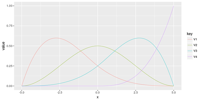
After encountering data sets too hefty for Gaussian Processes, I’ve been exploring splines and thought I’d start sharing some demos here. I’m indebted to others for much of this code, but hope to have made some worthwhile/clarifying additions for other newbies like myself. First up is the attached demo of a simple scenario of a single continuous predictor that compares sampling performance between a regular representation of the splines versus a sparse representation. As noted, the sparse representation has better performance when the number of splines is above about 100; for significantly fewer splines, the sparse version can be dramatically worse, presumably due to overhead somewhere.
spline_fit.r (8.4 KB)
spline_fit.stan (1.5 KB)
spline_fit_sparse.stan (1.8 KB)
Oh, and one thing on which I’d appreciate feedback is that I think in exploring this I discoveredt that the splines::bs() function (not a stan-related R package, I know) appends a column of zeros to the end of the spline matrix, so if you don’t notice and ask your model for as many coefficients as there are columns in that matrix, you end up having a final coefficient that is uninformed by any data, which presumably might slow down sampling. Anyone know why splines::bs() does this? Bug?
I don’t wont to figure it out, since there is a better way to specify the number of knots by
using the degree of freedom parameter:
bs(x, df=4, degree=3)
I have encountered the splines::bs behavior as well. I have got used to stripping the last column. It has something to do with whether you include boundary points as your knots. I also like using the df parameter, but this gives you a zero row :-D
To sum:
#Has zero first row
splines::bs(0:10,knots = c(5), degree = 3)
splines::bs(0:10, degree = 3, df = 4)
#Has zero last column
splines::bs(0:10,knots = c(0, 5, 10), degree = 3)
#Has zero first row AND last column
splines::bs(0:10,knots = c(5, 10), degree = 3)

#Has no zero row/columns
splines::bs(0:10,knots = c(0,5), degree = 3)
Isn’t that something like a sum-to-zero constraint? Anyway, if
you add a column of 1’s as Intercept, the design matrix has
full rank. It don’t see the problem at the moment.
rankMatrix(cbind(splines::bs(0:10, degree = 3, df = 4),1))
[1] 5
attr(,“method”)
[1] “tolNorm2”
attr(,“useGrad”)
[1] FALSE
attr(,“tol”)
[1] 2.442491e-15
