I am a relatively new user of Stan struggling with stable behavior of a model that works well with no problems in JAGS. I am wondering if the performance/behavior is linked somehow to the way I wrote the code in Stan. I would appreciate if you could help me with that problem.
The model contains regularly spaced missing observations, and both JAGS and San’s versions account for that.
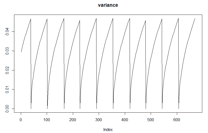
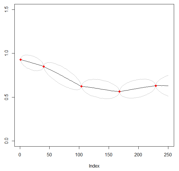
The variance between observations increases and collapses along with occurrence of the new, consequent observation.
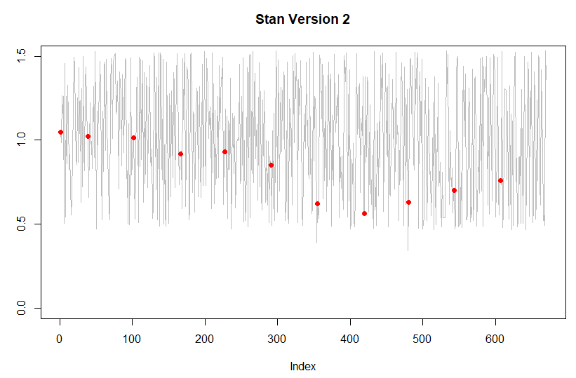
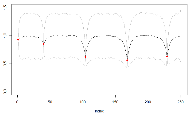
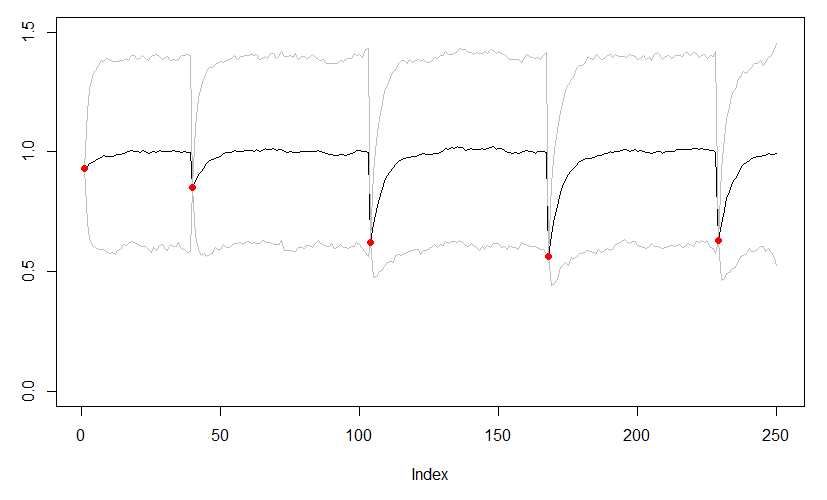
(in all plots gray lines represent 80% confidence interval)
Stan Model:
data {
  int<lower=1> N0;
  vector[N0] Factor1_0;
  int FCT1_NA_COUNT;
  int FCT1_NA_INDEX[FCT1_NA_COUNT];
  vector[N0] FACTOR1_SD;
}
parameters {
  vector<lower=0.3, upper=1.7>[FCT1_NA_COUNT] FCT1_MISSING;
}
transformed parameters {
  vector[N0] FACTORS;
  FACTORS = Factor1_0; FACTORS[FCT1_NA_INDEX] = FCT1_MISSING;
}
model {
  for(i in 2:N0){
        #FACTORS[i] ~ normal(FACTORS[i-1],0.04);			        //    Version 1
        FACTORS[i] ~ normal(FACTORS[i-1],FACTOR1_SD[i]); 	//    Version 2
  }
  }
Version 1 of the Stan’s code is relatively stable, fast and yields expected results (but not the results that I am trying to model). The 2nd version with the increasing variances (all are below 0.04) doesn’t converge, and simulations don’t produce the expected behavior (I’ll include some plots to present that.
If so, maybe try adding a bit of extra noise to maybe experiment and see if just being close to zero is causing numerical issues?
Can you post the data for this? I’m not seeing from the plots which data points you have and which are missing, which looks important for interpreting FACTOR1_SD.
Since the post talks about variance, I just want to make it clear that JAGS uses precision (inverse variance) and Stan uses scale (standard deviation) to parameterize the normal.
Can you share the JAGS version and data that converges? Why are the FCT1_MISSING given those hard interval bounds? Did you first try without that? That can be a real problem computationally and statistically if the missing values are consistent with values near the boundaries.
but you’d probably just want to just define FACTOR1_SD as not having that first element rather than having to slice it each time, given that it’s data. Or you could transform in transformed data to define:
transformed data {
  vector[N0 - 1] sigma = FACTOR1_SD[2:N0];

...
model {
  FACTORS[2:N0] ~ normal(FACTORS[1:N0 - 1], sigma);
Thanks for your time. I think this could be one of factors, but what I realized is that there is some problem with implementation of the model in Stan.
data {
int<lower=1> N0;
vector[N0] Factor1_0;
int FCT1_NA_COUNT;
int FCT1_NA_INDEX[FCT1_NA_COUNT];
vector[N0] FACTOR1_SD;
int<lower=1>N0_DATA;
int FACTOR1_DATA_IDX[N0_DATA];
Thank you for replying. I apply precision in JAGS, and the code is enclosed in my response to Ben.
FCT1_MISSING - my guess is that this is potentially the hart of the problem, but honestly I have some problems with correct implementation. One of versions:
data {
int<lower=1> N0;
vector[N0] Factor1_0;
int FCT1_NA_COUNT;
int FCT1_NA_INDEX[FCT1_NA_COUNT];
vector[N0] FACTOR1_SD;
int<lower=1>N0_DATA;
int FACTOR1_DATA_IDX[N0_DATA];
If you’re fitting a time series and want to get estimates of what is happening between points, usually this looks a lot more like a prediction sort of thing than a missing value thing.
So you fit a curve to all the red points and then predict the things in the middle.
Right now what is happening in the plots is kinda weird. Between the red points, the medians drift back to be near 1 and seem to ignore whatever data is on either side of them. This doesn’t seem like the usual assumption for time series.
Thank you for your response. I agree this looks very strange, and I would not expect to see that given the specification of the model .
The idea is to estimate points between the known observations (red dots), that are being used in evaluation of an integral in the later part of the code. The unobservable points are known by market participants to certain extent, as they are function of a monthly GNP and daily SP500 (knowing the direction of SP500 gives some idea of where the observable points can be).
I applied two other approaches:
regression using SP500 as an explanatory variable - deviations of the red dots from the median are too big to be of practical use.
I applied splines - in this case the model is fast if we have exactly the same number of days between observations, but in practice this is not the case as small differences in number of points between observations requires increasing max_treedepth - given complexity of the overall program this slows down the process substantially.
The most realistic model that I see here is presented in the 2nd plot from the top. Would you have some other suggestions of how to make that code in Stan working?
If the splines weren’t flexible enough, have you looked at GPs? Does the second picture in Figure 2.2 of http://www.gaussianprocess.org/gpml/chapters/RW2.pdf seem interesting? That looks similar to the second plot from the top and you can do this in closed form.
How many days of data and such? Is it 5 data points over 250 days?
What are your goals beyond just fitting this data?
The reason that your black lines curve up is because you’ve specified a prior on FCT1_MISSING in the range 0.3 to 1.7. This centre of this range is (0.3+1.7)/2 = 1.0, so you see that your prior encourages the lines to go towards 1.0.
Why do you have this prior?
If you simply remove the bounds on FCT1_MISSING and replace 0.2 with sigma, defined as a parameters real<lower=0> sigma then you’ll have a standard random walk model.
In the earlier post, I can’t understand why you pass FACTOR1_SD in as data, and similarly why you have a different standard deviation for every time point. How can you know this before in a way that’s consistent with your data points?
I think that you are confused about how a random walk is modelled. You don’t specify individual standard deviations for each point. The graph you’ve drawn first about the variance profile is not correct - the variance does not “collapse back to zero”. If your data follow a random walk then knowing a value at time T+1 places a constraint on the value at time T.
Have a look at Brownian bridge on Wikipedia - if you have a standard Brownian motion (ie continous time random walk where the value of the process is fixed at time 0 and time T) then the variance is t*(T-t)/T, a concave down parabola with values zero at times t and T. The variance is maximal half way between the two points. It looks nothing like the graph you have first shown.
Thank you again. This looks indeed very close to what I am looking for. I started working on the implementation, but I have also found figure 9 in the paper http://www.robots.ox.ac.uk/~sjrob/Pubs/philTransA_2012.pdf
but I ma not sure yet which kernel is capable of generating such process.
In filtering you make predictions about time t based on everything that came before. In smoothing you use information from both directions.
Plots of filtering effects can be kinda deceiving, cause they’re really plots of a bunch of different modes (one model including n points, one with n + 1, etc.). The smoothing models use all the data to inform all the inferences.
When you use GPs to interpolate data, they look like smoothers.
Apologies for the late response. I agree with the points you’ve raised. How do I know the prior have those limits - histrionically they’ve never been exceeded, and I would think that it is highly unlikely that they will ever be exceeded. Having said that 0.2 SD was unrealistic, for the purpose of the simulation, and I admit I was a little bit confused by this plot.
Increasing variance - I overlooked that, initially I tried to apply a simplified model using na.locf and increasing variances.
Works just find, and this is exactly what you expect for a random walk model.
You’re misunderstanding figure 9 in that paper that’s referred to. That’s talking about how the forecast prediction variance evolves UNTIL a data point is seen. That’s the behaviour you see to the right of the right most data point in the graph above. There’s a big difference between the likelihood of the model (ie that there is a random walk at each time step) and the posterior uncertainty. Figure 9 DOES NOT show the posterior uncertainty of the model at a given time step in the case when there is another data point to the right.
Read the caption on that figure: " The GP is run sequentially making forecasts until a new datum is observed. Once we make an observation, the posterior uncertainty drops to zero (assuming noiseless observations)". This figure describes the forecast behaviour in the absence of data vs when data exists.
Thank you. This yields exactly like one of my codes in JAGS. On the top of my transition to Stan, I had some problems with implementation of AR(1) with intercept for some reasons - the results I was getting definitely did not look right. Extending your code to AR(1) with intercept is straightforward and solves my problem.
The only discomfort I have here concerns increasing treedepth, but I guess nothing can be done to resolve this apart form increasing the treedepth above 10.
Warning messages:
1: There were 206 transitions after warmup that exceeded the maximum treedepth. Increase max_treedepth above 10.
IO use 4k warmup, 10k sims.
I agree this case requires a simple model. Thank you so much.