SBC for arma model

Hi all,

As mentioned in the stan dev call I’ve been running SBC on the benchmark models:

I’m using cmdstan called via a python script which calculates the SBC histograms for a given model. I’m using cmdstan / python rather than something like cmdstanpy as my objective is to use the script to verify SMC-Stan, which currently exists as a cmdstan fork.

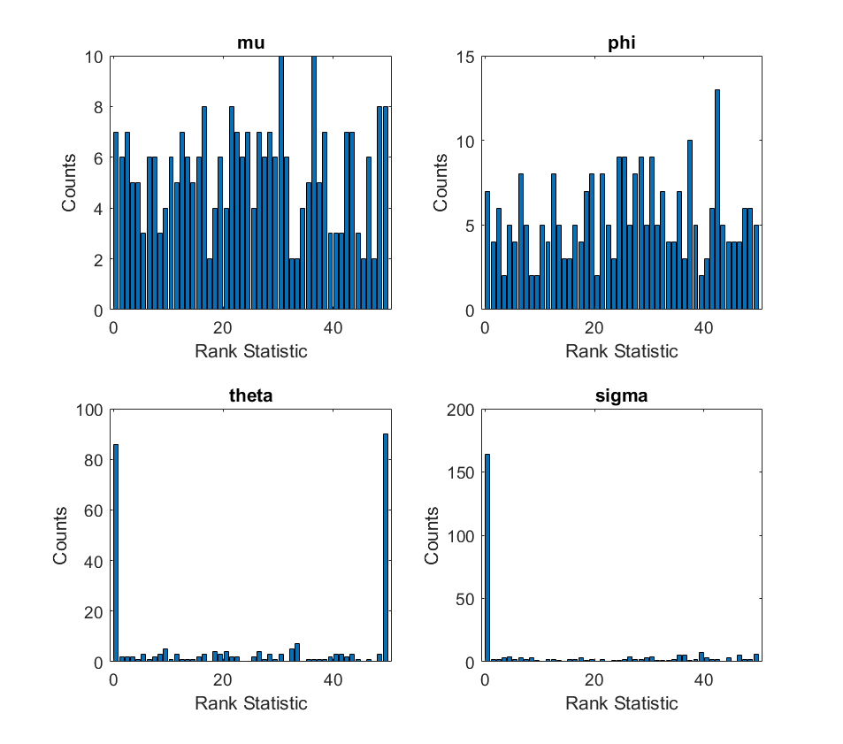
I managed to reproduce the results for the eight_schools model, but I’m seeing extremely skewed histograms for the arma model (shown below).

Here’s the model code I’m using:

// ARMA(1, 1)
functions {
  real half_cauchy_rng(real lb) {
    real p = cauchy_cdf(lb, 0, 2.5);
    real u = uniform_rng(p, 1);
    real y = 2.5*tan(pi()*(u - 0.5)); // inverse cauchy_cdf
    return y;
  }
}

data {
  int<lower=1> T; // number of observations
  real y[T];      // observed outputs
}

transformed data {
  real y_sim[T];
  real mu_sim;
  real phi_sim;
  real theta_sim;
  real<lower=0> sigma_sim;
  vector[T] nu_sim;  // prediction for time t
  vector[T] err_sim; // error for time t
  
  mu_sim = normal_rng(0, 10);
  phi_sim = normal_rng(0, 2);
  theta_sim = normal_rng(0, 2);
  sigma_sim = half_cauchy_rng(0);
  
  for (t in 1:T){
    err_sim[t] = normal_rng(0, sigma_sim);
  }
  
  nu_sim[1] = mu_sim + phi_sim * mu_sim; // assume err[0] == 0
  y_sim[1] = err_sim[1] + nu_sim[1];
  for (t in 2:T) {
    nu_sim[t] = mu_sim + phi_sim * y_sim[t - 1] + theta_sim * err_sim[t - 1];
    y_sim[t] = err_sim[t] + nu_sim[t];
  }
}

parameters {
  real mu;             // mean coefficient
  real phi;            // autoregression coefficient
  real theta;          // moving average coefficient
  real<lower=0> sigma; // noise scale
}

model {
  vector[T] nu;  // prediction for time t
  vector[T] err; // error for time t
  
  mu ~ normal(0, 10);
  phi ~ normal(0, 2);
  theta ~ normal(0, 2);
  sigma ~ cauchy(0, 2.5);
  
  nu[1] = mu + phi * mu; // assume err[0] == 0
  err[1] = y[1] - nu[1];
  for (t in 2:T) {
    nu[t] = mu + phi * y[t - 1] + theta * err[t - 1];
    err[t] = y[t] - nu[t];
  }
  
  err ~ normal(0, sigma);
}

generated quantities {
    int<lower=0,upper=1> lt_sim[4];
    lt_sim[1] = mu < mu_sim;
    lt_sim[2] = phi < phi_sim;
    lt_sim[3] = theta < theta_sim;
    lt_sim[4] = sigma < sigma_sim;
}

Does anyone have ideas as to what might be going on?

2 Likes

The first thing I check when I see such bad histograms is whether my simulation code actually matches the model.

If I understand the code correctly, you basically want to ignore y and simulate your own y_sim. It is therfore my impression that you want to be using y_sim instead of y in the model block…

BTW, an easier way to get half cauchy is IMHO simply fabs(cauchy_rng(...)), but that does not really matter.

Best of luck with the project!

1 Like

I can’t believe I didn’t see that, thanks @martinmodrak! I’ll re-run with the fixed model block. Also thanks for the tip for the half cauchy!

1 Like

No worries, happens to all of us :-D

Just thought I’d give an update as to where I got with this. With the fix in the model block the histograms look slightly less skewed but it still looks like the model-fitting is biased.

Here’s the updated model code:

// ARMA(1, 1)
functions {
  real half_cauchy_rng(real lb) {
    real p = cauchy_cdf(lb, 0, 2.5);
    real u = uniform_rng(p, 1);
    real y = 2.5*tan(pi()*(u - 0.5)); // inverse cauchy_cdf
    return y;
  }
}

data {
  int<lower=1> T; // number of observations
}

transformed data {
  real y_sim[T];
  real mu_sim;
  real phi_sim;
  real theta_sim;
  real<lower=0> sigma_sim;
  vector[T] nu_sim;  // prediction for time t
  vector[T] err_sim; // error for time t
  
  mu_sim = normal_rng(0, 10);
  phi_sim = normal_rng(0, 2);
  theta_sim = normal_rng(0, 2);
  sigma_sim = half_cauchy_rng(0);
  
  for (t in 1:T){
    err_sim[t] = normal_rng(0, sigma_sim);
  }
  
  nu_sim[1] = mu_sim + phi_sim * mu_sim; // assume err[0] == 0
  y_sim[1] = err_sim[1] + nu_sim[1];
  for (t in 2:T) {
    nu_sim[t] = mu_sim + phi_sim * y_sim[t - 1] + theta_sim * err_sim[t - 1];
    y_sim[t] = err_sim[t] + nu_sim[t];
  }
}

parameters {
  real mu;             // mean coefficient
  real phi;            // autoregression coefficient
  real theta;          // moving average coefficient
  real<lower=0> sigma; // noise scale
}

model {
  vector[T] nu;  // prediction for time t
  vector[T] err; // error for time t
  
  mu ~ normal(0, 10);
  phi ~ normal(0, 2);
  theta ~ normal(0, 2);
  sigma ~ cauchy(0, 2.5);
  
  nu[1] = mu + phi * mu; // assume err[0] == 0
  err[1] = y_sim[1] - nu[1];
  for (t in 2:T) {
    nu[t] = mu + phi * y_sim[t - 1] + theta * err[t - 1];
    err[t] = y_sim[t] - nu[t];
  }
  
  err ~ normal(0, sigma);
}

generated quantities {
    int<lower=0,upper=1> lt_sim[4];
    lt_sim[1] = mu < mu_sim;
    lt_sim[2] = phi < phi_sim;
    lt_sim[3] = theta < theta_sim;
    lt_sim[4] = sigma < sigma_sim;
}

I’m currently running SBC on the rest of the benchmark models. So far I’ve seen non-uniform histograms in a couple of other models, so it might be that I’m doing something wrong in my python script. I’ll upload the code to github and will post the results in a new thread.

2 Likes

One thing that’s potentially problematic (but I currently can’t think completely straight about this) is that the err ~ normal(0, sigma); in the model code actually might not correspond well to the err_sim[t] = normal_rng(0, sigma_sim); because err is a non-linear function of parameters and thus some Jacobian adjustment might be needed.

One thing that might be sensible and easy to implement would be to avoid computing err altogether and instead have y ~ normal(nu, sigma);

Also note that such big discrepancies should be visible just from one or two runs, so no need to waste time running full SBC to see if the change helps.

Some further ideas if that does not help: If you remove the likelihood, do you pass SBC? (you should, so that is the test of your infrastructure).

1 Like

Okay so I tried to see if this might be case by first eliminating the moving average term completely. Code and results are shown below.

// ARMA(1, 1)
functions {
  real half_cauchy_rng(real lb) {
    real p = cauchy_cdf(lb, 0, 2.5);
    real u = uniform_rng(p, 1);
    real y = 2.5*tan(pi()*(u - 0.5)); // inverse cauchy_cdf
    return y;
  }
}

data {
  int<lower=1> T; // number of observations
}

transformed data {
  real y_sim[T];
  real mu_sim;
  real phi_sim;
  real<lower=0> sigma_sim;
  vector[T] nu_sim;  // prediction for time t
  
  mu_sim = normal_rng(0, 10);
  phi_sim = normal_rng(0, 2);
  sigma_sim = half_cauchy_rng(0);
  
  nu_sim[1] = mu_sim + phi_sim * mu_sim;
  y_sim[1] = normal_rng(nu_sim[1], sigma_sim);
  for (t in 2:T) {
    nu_sim[t] = mu_sim + phi_sim * y_sim[t - 1];
    y_sim[t] = normal_rng(nu_sim[t], sigma_sim);
  }
}

parameters {
  real mu;             // mean coefficient
  real phi;            // autoregression coefficient
  real<lower=0> sigma; // noise scale
}

model {
  vector[T] nu;  // prediction for time t
  
  mu ~ normal(0, 10);
  phi ~ normal(0, 2);
  sigma ~ cauchy(0, 2.5);
  
  nu[1] = mu + phi * mu;
  for (t in 2:T) {
    nu[t] = mu + phi * y_sim[t - 1];
  }
  
  y_sim ~ normal(nu, sigma);
}

generated quantities {
    int<lower=0,upper=1> lt_sim[3];
    lt_sim[1] = mu < mu_sim;
    lt_sim[2] = phi < phi_sim;
    lt_sim[3] = sigma < sigma_sim;
}

So this gives the expected uniform histograms.

I then tried rewriting the original model to use y~normal(nu,sigma) instead and the problem returned (although interestingly, only for the parameters relating to the original err variable).

// ARMA(1, 1)
functions {
  real half_cauchy_rng(real lb) {
    real p = cauchy_cdf(lb, 0, 2.5);
    real u = uniform_rng(p, 1);
    real y = 2.5*tan(pi()*(u - 0.5)); // inverse cauchy_cdf
    return y;
  }
}

data {
  int<lower=1> T; // number of observations
}

transformed data {
  real y_sim[T];
  real mu_sim;
  real phi_sim;
  real theta_sim;
  real<lower=0> sigma_sim;
  vector[T] nu_sim;  // prediction for time t
  
  mu_sim = normal_rng(0, 10);
  phi_sim = normal_rng(0, 2);
  theta_sim = normal_rng(0, 2);
  sigma_sim = half_cauchy_rng(0);
  
  nu_sim[1] = mu_sim + phi_sim * mu_sim; // assume err[0] == 0
  y_sim[1] = normal_rng(nu_sim[1], sigma_sim);
  for (t in 2:T) {
    nu_sim[t] = mu_sim + phi_sim * y_sim[t - 1] + theta_sim * (y_sim[t-1] - nu_sim[t-1]);
    y_sim[t] = normal_rng(nu_sim[t], sigma_sim);
  }
}

parameters {
  real mu;             // mean coefficient
  real phi;            // autoregression coefficient
  real theta;          // moving average coefficient
  real<lower=0> sigma; // noise scale
}

model {
  vector[T] nu;  // prediction for time t
  
  mu ~ normal(0, 10);
  phi ~ normal(0, 2);
  theta ~ normal(0, 2);
  sigma ~ cauchy(0, 2.5);
  
  nu[1] = mu + phi * mu; // assume err[0] == 0
  for (t in 2:T) {
    nu[t] = mu + phi * y_sim[t - 1] + theta * (y_sim[t-1] - nu[t-1]);
  }
  
  y_sim ~ normal(nu, sigma);
}

generated quantities {
    int<lower=0,upper=1> lt_sim[4];
    lt_sim[1] = mu < mu_sim;
    lt_sim[2] = phi < phi_sim;
    lt_sim[3] = theta < theta_sim;
    lt_sim[4] = sigma < sigma_sim;
}

So at the moment I’m kind of at a loss as to why this is happening!

(Also thanks for the other tips, I tried with the likelihood removed and that also passed the test.)

1 Like

Just one more basic thing to check: are all your diagnostics in all runs all right? (divergences, neff, Rhat) When I do SBC, I usually have to set much narrower priors than I would in application to avoid producing large number of extreme datasets that than cause problems for the sampler. I’ve definitely had SBC runs where >80% of the fits did not converge purely because the datasets were extreme, while the model was basically OK. And when that happens the histograms can look very bad. You have pretty wide priors, so I wouldn’t be surprised if that at least partly plays a role.

Practically, what I do is to record the number of divergences, lowest n_eff and largest Rhat for each fit and then look at the proportion of fits that fail at least one diagnostic.

3 Likes

@martinmodrak This is a good point. Most of the diagnostics are unavailable as I’m running everything on a single-chain basis. I had assumed since the benchmark models have been extensively tested that there shouldn’t be any issues, but that only applies for the given datasets.

I’ve also since realised that it isn’t necessary to do SBC with single independent chains, so my plan is to do a multiple-chain implementation and then I can look at things like Rhat. I can then hopefully look for non-convergence and other pathologies.

I would expect all diags to actually be available. Divergences are definitely accessible, but you can also definitely compute ESS and Rhat for single chains - it is less sensitive, but the code works (at least the R implementation), e.g. this works:

single_chain <- matrix(rnorm(100), nrow = 100, ncol = 1)
posterior::rhat(single_chain)
#> [1] 1.024309
posterior::ess_bulk(single_chain)
#> [1] 97.23252
1 Like

2 posts were split to a new topic: Using narrower priors for SBC

I tried running stansummary and diagnose from CmdStan and indeed it does provide diags for a single chain. Not sure why I got it into my head that it didn’t!

In any case I’ll update the SBC code to make sure these diagnostic checks are being passed.