Sampling cannot pass warm-up stage for piece-wise likelihood

I am doing a simulation study for my multiple quantile regression model that involves fitting a piece-wise likelihood. Following is my problem set up:

\begin{aligned} f_Y(y|\mathbf{x_i})&=\begin{cases} \frac{1}{\mathbf{x}_i^T\mathbf{\alpha}_1}f_0\left(\frac{y}{\mathbf{x}_i^T\mathbf{\alpha}_1}\right), \ q(\kappa_0|\mathbf{x}_i)<y\le q(\kappa_1|\mathbf{x}_i)\\\\ \frac{1}{\mathbf{x}_i^T\mathbf{\alpha}_l}f_0\left(\frac{y-q(\kappa_{l-1}|\mathbf{x}_i)+\mathbf{x}_i^T\mathbf{\alpha}_lq_0(\kappa_{l-1})}{\mathbf{x}_i^T\mathbf{\alpha}_l}\right), \ q(\kappa_{l-1}|\mathbf{x}_i)<y\le q(\kappa_l|\mathbf{x}_i) \end{cases} \end{aligned}

where 0=\kappa_0<\kappa_1<\dots<\kappa_{L-1}<\kappa_L=1 are breakpoints representing multiple quantiles, and

\begin{equation} q(\tau|\mathbf{x}_i) = \sum_{l=1}^{L}\mathbf{x}_i^T\mathbf{\alpha}_lB_{l}(\tau) \end{equation}

is the proposed nonlinear true quantile process. \alpha_l=\begin{pmatrix}\alpha_{0l}\\\alpha_{1l}\end{pmatrix} is a vector of two elements for every l.


In order to ensure the monotonicity of quantiles, I generate \alpha_l^* first and then apply restrictions to form \alpha_l. My priors are

\begin{align*} \alpha^*_{0l}\overset{i.i.d}{\sim} \mathcal{N}(\mu_0,\tau_0), \ \alpha^*_{1l}\overset{i.i.d}{\sim} \mathcal{N}(\mu_1,\tau_1), \ \mu_j\overset{i.i.d}{\sim}\mathcal{N}(0,c), \ \tau_j\overset{i.i.d}{\sim} \gamma(a,b) \end{align*}

and \alpha_l^* is further transformed to \alpha_l using a self-defined function.


Case 1: L=2, \kappa_1=0.5, f_0\sim \phi, i.e. a nonlinear median regression. The goal is to recover \alpha_l, l =1,2.

\begin{aligned} f_Y(y|\mathbf{x}_i)&=\begin{cases}\frac{1}{\mathbf{x}_i^T\mathbf{\alpha}_1}\phi(\frac{y}{\mathbf{x}_i^T\mathbf{\alpha}_1}),\ y\le 0\\\\ \frac{1}{\mathbf{x}_i^T\mathbf{\alpha}_2}\phi(\frac{y}{\mathbf{x}_i^T\mathbf{\alpha}_2}),\ y> 0\end{cases}\\\\ \end{aligned}
functions{
    matrix thresh(matrix alpha_star, real eps){
      int M = rows(alpha_star);
      int N = cols(alpha_star);
      matrix[M,N] alpha_out;
      for(l in 1:N){
        real WC = alpha_star[1,l]-sum(fabs(alpha_star[2:M,l]));
        if(WC < eps){
          alpha_out[1,l] = eps;
          alpha_out[2:M,l] = rep_vector(0,M-1);
        }else{
          alpha_out[,l] = alpha_star[,l];
        }
      }
      return alpha_out;
    }
    int which_less(row_vector q_vec, real a){
      int loc = 1;
      while((loc<=num_elements(q_vec))&&(q_vec[loc]<a)){
        loc += 1;
      }
      return loc-1;
    }
}
data {
  int<lower=0> N;
  int L;
  vector[N] y;
  matrix[N,2] x;
  matrix[L,L-1] basis_m;
  vector[L-1] q_base;
}

// The parameters accepted by the model. Our model
// accepts two parameters 'mu' and 'sigma'.
parameters {
  vector[2] mu;
  matrix[2,L] alpha_star;
  vector<lower=0> [2] prec;
}

transformed parameters{
  vector<lower=0> [2] sigma;
  matrix[2,L] alpha;
  for(j in 1:2){
    sigma[j] = 1/sqrt(prec[j]);
  }
  alpha = thresh(alpha_star,0.1);
}

model {
  matrix[N,L] x_a;
  matrix[N,L-1] q_model;
  mu ~ normal(0,10);
  prec ~ gamma(0.3,0.3);
  for(j in 1:2){
    alpha_star[j,] ~ normal(mu[j],sigma[j]);
  }
  x_a = x*alpha;
  q_model = x_a*basis_m;
  for(i in 1:N){
    if(y[i]<=q_model[i,1]){
       y[i] ~ normal(0,x_a[i,1]) T[,q_model[i,1]];
    }else{
      if(y[i]>q_model[i,L-1]){
        y[i] ~ normal(q_model[i,L-1]-x_a[i,L]*q_base[L-1],x_a[i,L]) T[q_model[i,L-1],];  
      }else{
        int idx = which_less(q_model[i,],y[i]);
        y[i] ~ normal(q_model[i,idx]-x_a[i,idx+1]*q_base[idx],x_a[i,idx+1]) T[q_model[i,idx],q_model[i,idx+1]];
      }
    }
  }
}

I first generate a random design matrix and then generate true quantile process based on the design matrix. For this case the model did a perfect job recovering the parameters of interest.


Case 2: L=4, \kappa_1=0.25,\kappa_2=0.5,\kappa_3=0.75,f_0\sim \phi, i.e. a nonlinear multiple quantile regression. The goal is again to recover \alpha_l, l =1,2,3,4. I used the same code and simulation procedure as listed above, but this time the results are really bad.

First of all, the sampling is really inefficient. With 1000 iterations, 250 warm-up it takes minutes whereas only seconds is needed in the first case. Secondly, nearly all transitions reach the default maximum tree depth (10) and the traceplot displays high autocorrelation. Lastly, when I attempt to increase the maximum tree depth from 10 to 30, the program just will not start or finish warm-up stage even after hours.

I have tried hours to detect and fix problems in my model and coding but there hadn’t been any improvement. Do you guys see any obvious problems from the model or code ? What are some guidelines to diagnose my model in this case. I really appreciate any help.

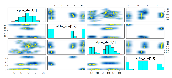
Sorry I didn’t have time to look at the model, but wanted to comment that treedepth 30 means 10^30 leapfrog steps, which is a lot. Couple quick suggestions: 1) check the stepszie: piecewise is problematic for HMC and it’s likely that stepsize in adaptation gets very small, 2) check if there are trends in chains: this could indicate some non-identfiablity in your model.

Hi Aki,

Thanks for your suggestions. I checked the stepsize and it’s indeed the case. It got to as small as 10^-6 during warmup. I also suspected that there were some non-identifiability in my model. Is there a quick way to detect which parameters are non-identifiable? What kind of trends should I be looking at?
I have attached the traceplot for one of my parameter and pairs plot for several of them. Most of the parameters clearly got stuck at initial values, I did not receive a warning of divergence but only maxtreedepth.

Uh, that looks bad.

Can you plot how your piecewise likelihood looks like? That is likely the problem.
Do you have priors on all parameters?

A shameless plug: Identifying non-identifiability
(discusses some quite different situations, but hopefully will give you some ideas)

1 Like

For a specific design vector \mathbf{x} and parameter matrix \alpha, the likelihood of y looks like the following


In general for each \mathbf{x} the likelihood consists of 4 pieces of truncated normal distributions. I did specify priors for all parameters.

Hi Martin,

Thanks for sharing this. I will try to see if I can find any similarities of the diagnostics.

HMC in Stan works only for continuous densities (derivative should also exist everywhere, but it may produce useful sample with small bias if discontinues in derivative are small) and this likelihood produces posterior density which is far from continuous. Only way to use this likelihood in Stan is to do the model in pieces.

For each y_i, I check which piece it falls into, and then model that y_i as a truncated normal accordingly. Is this equivalent to your modelling by piece?

Another potential issue might be that my \alpha parameter affects the breakpoint, center and scale. Maybe this makes the model non-identifiable?

If the y values are observed this should be fine. For HMC the likelihood needs to be continuous in terms of the parameters. The problem I see is that the thresh function is not continuous enough. Could you make it more continuous?

Since \mathbf{x}_i^T\alpha_l plays the role as a standard deviation for each l and I assigned unconstrained prior on \alpha_l, I need to transform \alpha_l such that \mathbf{x}_i^T\alpha_l>0. Right now I am assuming that the design matrix is N\times\ 2 and the entries of the second column is within [-1,1]. Since the entries of the first column are all 1, I only need to ensure that \alpha_{1,l}-|\alpha_{2,l}|>0. Maybe I can change thresh function to do \alpha_{1,l}=|\alpha_{2,l}|+\epsilon, this will get rid of the if conditions. The absolute function is still there though.