Regression Models for Duration Data

[carlocav]

I am fitting brms models on duration data representing the number of days of delay in paying invoices from the expiration date (negative values represents advance payments). The data consists of some exploratory variables such as the customer, invoice amount, revenue type, expiry month, ecc.

The main goal is to do predictions, but instead of a point estimate I need a reliable probability distribution of the outcome (i.e. days of delay) on new invoices, that’s why I am using Bayesian tools.

I removed from the training set observations having values for the outcome variable in the first and the last decile since they complicate the estimation process bringing the models to return worse forecasts on new invoices in the test set. After doing this the response variable ranges from -15 to 103.

This is the initial distribution of the outcome, as you can see it is bimodal:

Below is the distribution of the response on the data that I am using to fit the models.
As I said before, I removed data where the response takes values < -15 or >103 (1st and 9th deciles).

Since the distribution is positively skewed and has a lot of over-dispersion (mean is ~15.4, variance is 437), as a purely practical matter I tried to model the data with Negative Binomial, even if I don’t have count data.
In order to to this I had to make all the values of the outcome greater or equal to 0 removing the minimum observed value (-15).

blm_nb_2_prior <- c(set_prior("normal(0,1)", class = "b"),
                 set_prior("normal(0,10)", class = "Intercept", coef = ""),
                 set_prior("exponential(1)", class = "shape"))
blm_nb_2 <- brm(ritardo ~ ., data = train_juiced_shift, family = negbinomial(), prior = blm_nb_2_prior)

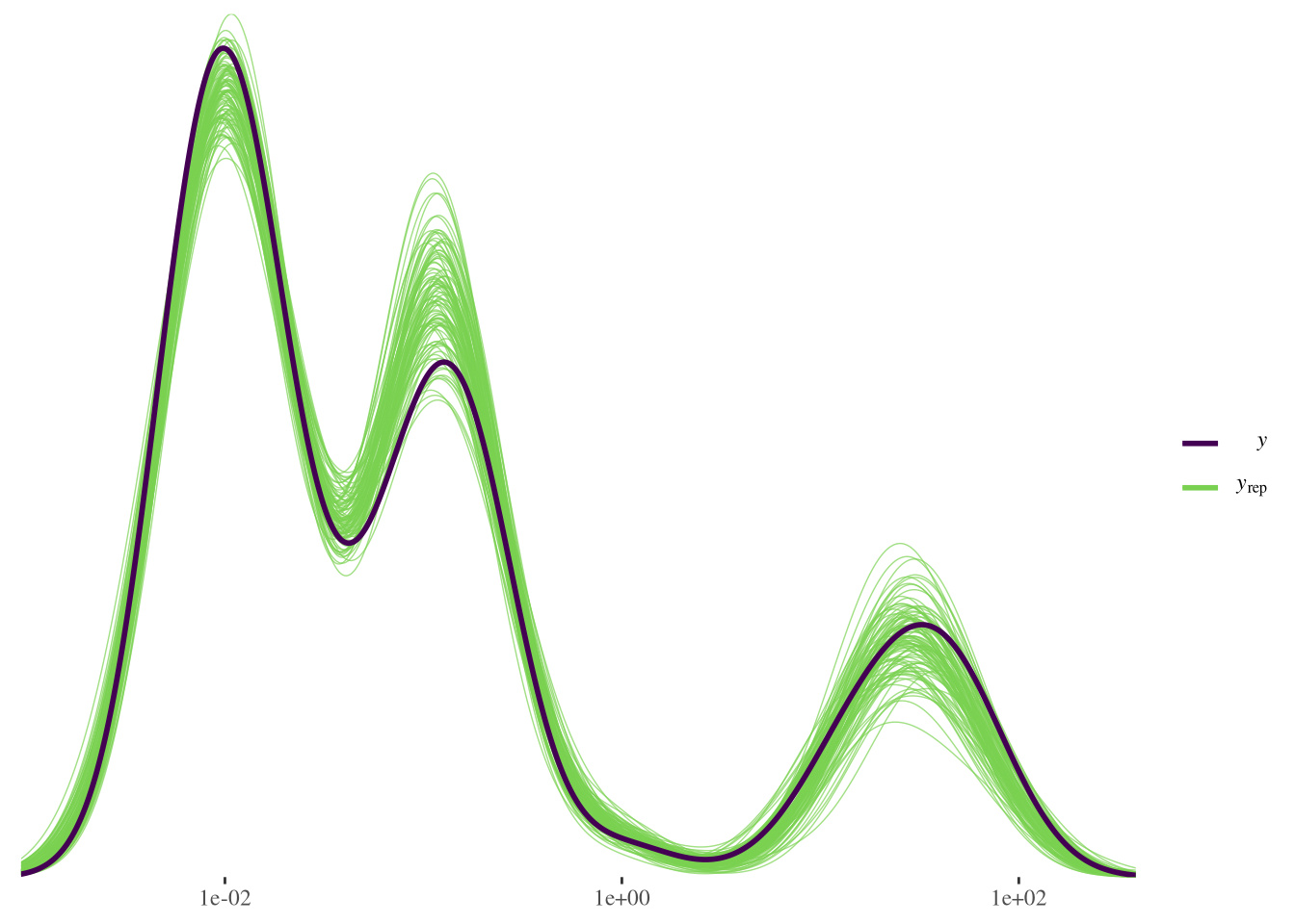
Below posterior predictive checks:

I also tried Weibull regression, which should be more suitable for time-to-event data:

brm(ritardo ~ ., family = weibull(), data = train_juiced_shift_2, chains = 4, cores = 4)

Loo comparison suggests Negative Binomial model is the best of the 2:

     elpd_diff se_diff

blm_nb_2 0.0 0.0
blm_w -226.1 12.1

To evaluate the effectiveness of the models on new data (not used to train the models and including those with the outcome variable taking “extreme” values i.e. inside the first or last decile), I also computed performance indicators such as RMSE, MAE, MDAE on the test set (comparing the median of the posterior distributions on the original scale with the actual values). According to this analysis, the best model among the 2 still is the NB, but the difference is small.

I ask you if is there is another model family that I could try that might work better on these duration data, maybe better suited to bimodal data and/or that can be fitted on the original data or removing less than 20% ​​of observations having extreme values.

[di4oi4]

I am just a novice here.

They also seem to be zero inflated variables. Maybe to consider zero-inflated negative binomial (family = zero_inflated_negbinomial()? Values <0 should be recoded into zeros. This should give you two outputs:

1. Which predictors were associated with receiving the salary on time (logistic regression or binomial part).
2. Which predictors were associated with a delay (negbinomial model).

[carlocav]

Thanks d14oi4 for your answer.

I am trying zero-inflated negative binomial, but unfortunatly this solution doesn’t allow to estimate how much in advance an invoice is paid (in case of negative delay i.e. advance payment).
About 35% of the observations have negative values for the outcome variable, which make up a set of very different situations (a value of -1 has a different meaning than a value of -10 or -50).

Maybe I could try time-to-event or mixture models?

Edit: Zero-inflated NB (recoding values <0 into zeros) is worse than NB and Weibull (removing extreme values so that delay ranges from -15 to 103, subtracting -15 so that values are all positive and after having fitted the model and made the predictions adding up 15 to the posterior distributions).

[scholz]

Hi @carlocav,

@carlocav

I removed from the training set observations having values for the outcome variable in the first and the last decile since they complicate the estimation process bringing the models to return worse forecasts on new invoices in the test set.

Not sure about this. After all, you remove some uncertainty that does exist in the real world process producing the data. However, I am not experienced with building models optimized for predictions so maybe that is the right thing to do.

For your likelihood functions, you should probably stick to discrete ones if your outcomes are integers or transform your outcomes. If negative values in your outcome are a problem, you could try to transform it to represent days since invoice if possible.
You could try both the exgaussian and shifted_lognormal likelihoods for reaction times. That sounds like it would fit the process.
Alternatively, you could try out a mixture model, eg 2 negative binomials (examples).

Good luck

[carlocav]

Thank you very much @scholz for your answer.

For your likelihood functions, you should probably stick to discrete ones if your outcomes are integers or transform your outcomes.

So it is better to make a transformation before fitting exgaussian, shifted_lognormal and the mixture model? In case which transformation do you suggest?
Among these 3 models only the mixture can generate bimodal posterior distributions right?

[scholz]

@carlocav

So it is better to make a transformation before fitting exgaussian, shifted_lognormal and the mixture model?

You could try it without a transformation and use loo to compare with the other models. After all, you can just round the predictions the model gives you in the end.
The only transformation that I know that gives you positive values would be exp and logistic and both would be problematic in your case I think.

@carlocav

Among these 3 models only the mixture can generate bimodal posterior distributions right?

I think you should be able to fit 2 modes without mixtures. Could depend on the models though, I’m not sure here.
This is a shifted lognormal model I tried for one of my projects.

As you can see it could fit 2 modes but can’t handle the third. A mixture with 2 components can fit 3 modes because you get 1 mode per component and the third from the combination of the two.
This is the result for a mixture of 2 shifted lognormals that could handle all 3 modes.

[carlocav]

Thanks @scholz you are very helpful!
It looks like Shifted Log-Normal is slightly better than Negative Binomial (according to loo comparison and performance metrics on the test set), but still does not fit 2 modes on my data:

So I am trying a mixture of 2 Shifted Log-Normal, but I can’t get the convergence using this code:

mix <- mixture(shifted_lognormal, shifted_lognormal)
blm_mixslog_prior <- c(
  set_prior("normal(0,1)", class = "b"),
  set_prior("normal(0,10)", class = "Intercept", coef = "")
  )
blm_mixslog <- brm(ritardo ~ ., data = train_juiced_shift_2, family = mix, inits = 0)

Do you have any ideas to specify an a priori distribution that can help or whatever?

[scholz]

@carlocav

but still does not fit 2 modes on my data

This probably depends on the model. I’m not sure what the ~ . does exactly. In my case, I had a few population-level effects and two varying intercepts.

You can run your model with sample_prior = "only, and then use the pp_check function to look at how your prior looks. Maybe you are way off on something. My guess would be, that at least the intercept prior is too wide.
In my case, it also helped to give the different mixture components different intercept priors to clearly separate the chains.
As a starting point for how to specify those priors for the mixture, here is what I used. The values probably won’t work for you but it might help with the structure.

    prior(normal(-2, 2), class = "Intercept", dpar = "mu1"),
    prior(normal(2, 2), class = "Intercept", dpar = "mu2"),
    prior(normal(0, 4), class = "b", dpar ="mu1"),
    prior(normal(0, 4), class = "b", dpar ="mu2"),
    prior(uniform(0, 0.005), class = "ndt1"),
    prior(uniform(0, 210), class = "ndt2"),
    prior(gamma(0.1, 0.01), class = "sd", dpar = "mu1"),
    prior(gamma(0.1, 0.01), class = "sd", dpar = "mu2"),
    prior(gamma(0.1, 0.01), class = "sigma1"),
    prior(gamma(0.1, 0.01), class = "sigma2")

Finally, it can help to look at the trace plots with plot(blm_mixslog) to see what kind of sampling problems there are. In my case, I sometimes had chains that would sample well for their component and then jump to a second value. That lead me to separate the intercepts.

[carlocav]

I am trying fitting the mixture model following your advices.

This probably depends on the model. I’m not sure what the ~ . does exactly. In my case, I had a few population-level effects and two varying intercepts.

~ . means that use all the variables available in data as population-level effects. I have not tried Multilevel models (although I’d like to try them) because I don’t think I have groups/clusters of observations to be able to include varying effects

[carlocav]

Mixture of 2 Shifted Log-Normal looks promising:

Basically I used the prior distribution you suggested:

blm_mixslog_prior <- c(
  set_prior("normal(-1,3)", class = "Intercept", dpar = "mu1"),
  set_prior("normal(2,3)", class = "Intercept", dpar = "mu2"),
  set_prior("normal(0,1)", class = "b", dpar = "mu1"),
  set_prior("normal(0,1)", class = "b", dpar = "mu2"),
  set_prior("gamma(0.1, 0.01)", class = "sigma1"),
  set_prior("gamma(0.1, 0.01)", class = "sigma2")
)

Now I have to solve big sampling problems (r_hat > 1.5 for almost all parameters) trying to modify the apriori distribution following your advices.

[scholz]

@carlocav

Now I have to solve big sampling problems (r_hat > 1.5 for almost all parameters) trying to modify the apriori distribution following your advices.

Have you looked at the trace plots? You should be able to see sampling problems there. Could be priors that are set too wide/narrow/at the wrong place.
From a first glance, the ndt won’t work for you i’d think. It is the shift of the shifted lognormal and looking at your data, you need different numbers than what I used.

[carlocav]

Yes but I still struggle to understand how to change the a priori distributions on mixture models.
I think I am far from convergence, e.g.

The estimated distributions of the 2 intercepts are almost equal even if the mean of the prior distributions have opposite sign.

Also the parameters of the regressors do not converge but perhaps by adjusting these, they adjust accordingly

[gsinha]

Hi carlocav:

Not sure how you are handling “censoring” in this type of data. For example, do you have a full set of complete lifetimes i.e., where every invoice past its due date has been paid, or are there outstanding invoices that are yet to be paid. In this case, their lifetimes are censored, and these need to be properly accounted for in the likelihood function. I’m pretty sure brms allows you to fit these types of models as well.

[carlocav]

Hi @gsinha I have not problems of censored, every invoice has been paid. But as I wrote in the first message I had to remove about 20% of observations with extreme delays in order to fit a negative binomial model which turns into decent forecasts. Maybe using a more flexible model such as the mixture of shifted Log Normal I will be able to include also those observations, when I will be able to solve the giant sampling problems :)

[scholz]

You can see that in some of the trace plots both chains have two modes around the same values.
You could either go back to your data and base the priors for the two components on what you think represents the two processes resulting in the two modes or base the values on where the chains are focusing.
However, I think this would be considered basing your priors on your data. Usually that is not what you want to do but if all you want are predictions, it might be ok?

[carlocav]

Hi scholz
I tried to base the values on where the chains are focusing, which leads to this prior:

blm_mixslog_prior <- c(
  set_prior("normal(4,0.5)", class = "Intercept", dpar = "mu1"),
  set_prior("normal(4.7,0.5)", class = "Intercept", dpar = "mu2"),
  set_prior("normal(0,1)", class = "b", dpar = "mu1"),
  set_prior("normal(0,1)", class = "b", dpar = "mu2"),
  set_prior("gamma(1.5, 17)", class = "sigma1"),
  set_prior("gamma(24, 30)", class = "sigma2")
)

I was unable to add priors for ndt1 and ndt2 parameters, looking at the chains I tried e.g.

set_prior(“uniform(0, 0.01)”, class = “ndt1”)
set_prior(“uniform(0.9, 1.1)”, class = “ndt2”)

but I always end up in this error:

I also specified mixing proportions according to the values of the chains (0.46 and 0.54):

brm(bf(ritardo ~ ., theta1 = 0.46, theta2 = 0.54),… )

The chains looks better than before, but I still have some problems mainly on mu2_Intercept, mu1_Intercept, sigma1, ndt2:

I think I have yet to understand how to define a priori distributions for mixture models, but It looks like they are the only ones flexible enough to fit my data.