Real vs Vector parameter(s): one is working and the other is not (as expected). Why?

Hello, there. I am implementing a one-way linear mixed-effects model in rstan.

Y_{ij}=\mu+\sigma (t_i+b_j)+\epsilon_{ij},\quad\epsilon_{ij}\overset{\text{i.i.d.}}{\sim}\mathcal{N}(0,\sigma^2),\quad\text{for }i=1,\dotsb,a;\ j=1,\dotsb,n,

where \mu is the grand mean, t_i is the standardized treatment effects, b_j is the standardized subject-specific random effects, a is the number of levels, n is the number of subjects. Such a statistical model is often used in the within-subject (repeated measures) designs, e.g., Rouder et al. (2012 & 2017).

The priors are
(1) \pi(\mu,\sigma^2)\propto\sigma^{-2} (Jeffreys prior),
(2) t_i\mid g_t\overset{\text{i.i.d.}}{\sim}\mathcal{N}(0,g_t),
(3) g_t\sim\text{Scale-inv-}\chi^2(1,h_t^2),
(4) b_j\mid g_b\overset{\text{i.i.d.}}{\sim}\mathcal{N}(0,g_b),
(5) g_b\sim\text{Scale-inv-}\chi^2(1,h_b^2).
And, one effect is independent of another. The marginal prior for b_j's (or t_i's) is multivariate Cauchy.

My current working Stan model file is

data {
  int<lower=1> N;        // number of subjects
  int<lower=2> C;        // number of conditions
  vector[C] Y[N];        // responses
  real<lower=0> ht;      // scale parameter of the standardized treatment effects
  real<lower=0> hb;      // scale parameter of the standardized subject-specific random effects
}

parameters {
  real mu;              // grand mean
  real<lower=0> sigma;  // standard deviation of the error
  real<lower=0> gt;     // variance of the standardized treatment effects
  real<lower=0> gb;     // variance of the standardized subject-specific random effects
  vector[C] t;          // standardized treatment effects
  vector[N] b;          // standardized subject-specific random effects
}

transformed parameters {
  real<lower=0> eta;    // sd of the treatment effects
  real<lower=0> tau;    // sd of the subject-specific random effects
  eta = sigma * sqrt(gt);
  tau = sigma * sqrt(gb);
}

model {
  // linear mixed-effects model
  for (i in 1:N) {
    Y[i] ~ normal(mu + t + b[i], sigma);
  }
  t ~ normal(0, eta);
  b ~ normal(0, tau);

  // priors
  // mu ~ implicit uniform prior     // Jeffreys prior
  target += -2* log(sigma);          // Jeffreys prior
  gt ~ scaled_inv_chi_square(1, ht);
  gb ~ scaled_inv_chi_square(1, hb); // Rouder et al. (2012)
}

Plus, the R script (data source) is

mat <- matrix(c(10,6,11,22,16,15,1,12,9,8,
                13,8,14,23,18,17,1,15,12,9,
                13,8,14,25,20,17,4,17,12,12), ncol = 3,
              dimnames = list(paste0("s", c(1:10)),
                              c("Level1", "Level2", "Level3")))

datlist <- list(Y = mat, C = 3, N = 10, ht = 0.5, hb = 1)
model1 <- rstan::stan_model(file.choose())

mcmc <- rstan::sampling(model1, data = datlist, 
                        pars = c("mu", "sigma"), refresh = 0,
                        warmup = 200, iter = 2200, chains = 2)
rstan::summary(mcmc)

The code runs without warnings. Eventually, I want to extend the model to a heteroscedastic case, i.e., the error variance \sigma_i^2 is not constant across the different levels of the treatment. Hence, the variable sigma becomes a vector instead of a real number.

data {
  int<lower=1> N;        // number of subjects
  int<lower=2> C;        // number of conditions
  vector[C] Y[N];        // responses
  real<lower=0> ht;      // scale parameter of the standardized treatment effects
  real<lower=0> hb;      // scale parameter of the standardized subject-specific random effects
}

parameters {
  real mu;                   // grand mean
  vector<lower=0>[C] sigma;  // standard deviations of the error
  vector<lower=0>[C] gt;     // variances of the standardized treatment effects
  real<lower=0> gb;          // variance of the standardized subject-specific random effects
  vector[C] t;               // standardized treatment effects
  vector[N] b;               // standardized subject-specific random effects
}

transformed parameters {
  vector<lower=0>[C] eta;     // sds of the treatment effects
  real<lower=0> tau;          // sd of the subject-specific random effects
  real<lower=0> sigma_pooled; // pooled sd of the error (geometric mean)
  sigma_pooled = exp(sum(log(sigma))/C);
  eta = sigma_pooled * sqrt(gt);
  tau = sigma_pooled * sqrt(gb);
}

model {
  // linear mixed-effects model
  for (i in 1:N) {
    Y[i] ~ normal(mu + t + b[i], sigma);
  }
  t ~ normal(0, eta);
  b ~ normal(0, tau);

  // priors
  // mu ~ implicit uniform prior     // Jeffreys prior
  target += -2* log(sigma_pooled);   // Jeffreys prior
  gt ~ scaled_inv_chi_square(1, ht);
  gb ~ scaled_inv_chi_square(1, hb); // Rouder et al. (2012)
}

Ideally, the new code should conduct the same work as the previous one in a case of homoscedasticity. However, the console presents some warnings such as “There were 178 divergent transitions after warmup.”.

Any comments on this modeling issue are much appreciated. Thanks.
There is a mistake in coding the variance of the treatment effects. The following Stan model has been updated, but the warning messages still exist.

data {
  int<lower=1> N;        // number of subjects
  int<lower=2> C;        // number of conditions
  vector[C] Y[N];        // responses
  real tcrit;            // critical value
  real<lower=0> ht;      // scale parameter of the standardized treatment effects
  real<lower=0> hb;      // scale parameter of the standardized subject-specific random effects
}

parameters {
  real mu;                           // grand mean
  vector<lower=0>[C] sigma;          // error standard deviations
  real<lower=0> gt;                  // variance of the standardized treatment effects
  real<lower=0> gb;                  // variance of the standardized subject-specific random effects
  vector[C] t;                       // treatment effects
  vector[N] b;                       // subject-specific random effects
}

transformed parameters {
  real<lower=0> esd;         // geometric mean of the error sd
  real<lower=0> eta;         // sd of the treatment effects
  real<lower=0> tau;         // sd of the subject-specific random effects
  esd = exp(sum(log(sigma))/C);
  eta = esd * sqrt(gt);
  tau = esd * sqrt(gb);
}

model {
  // linear mixed-effects model
  for (i in 1:N) {
    Y[i] ~ normal(mu + t + b[i], sigma);
  }
  t ~ normal(0, eta);
  b ~ normal(0, tau);

  // priors
  // mu ~ implicit uniform prior           // Jeffreys prior
  target += -2 * sum(log(sigma));          // Jeffreys prior
  gt ~ scaled_inv_chi_square(1, ht);
  gb ~ scaled_inv_chi_square(1, hb);       // Rouder et al. (2012)
}

Hierarchical models can easily encounter divergences because they can induce some tricky posterior geometry more information in the User’s Guide.

Try using the non-centered parameterisation by changing your parameter specifications for t and b to:

  vector<multiplier=exp(sum(log(sigma))/C) * sqrt(gt)>[C] t;                       // treatment effects
  vector<multiplier=exp(sum(log(sigma))/C) * sqrt(gb)>[N] b;                       // subject-specific random effects

Thank you, Dr. Johnson. I am glad to learn the non-center trick. However, it does not seem to remedy the divergence situation.

Warning messages:
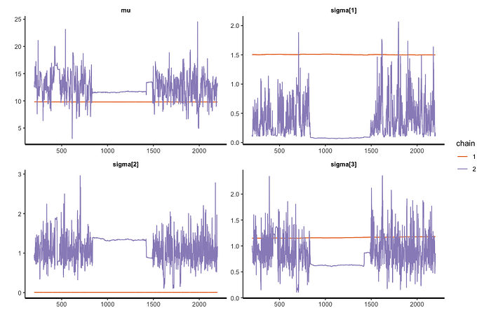
1: There were 2274 divergent transitions after warmup. See
https://mc-stan.org/misc/warnings.html#divergent-transitions-after-warmup
to find out why this is a problem and how to eliminate them. 
2: Examine the pairs() plot to diagnose sampling problems
 
3: The largest R-hat is 2.17, indicating chains have not mixed.
Running the chains for more iterations may help. See
https://mc-stan.org/misc/warnings.html#r-hat 
4: Bulk Effective Samples Size (ESS) is too low, indicating posterior means and medians may be unreliable.
Running the chains for more iterations may help. See
https://mc-stan.org/misc/warnings.html#bulk-ess 
5: Tail Effective Samples Size (ESS) is too low, indicating posterior variances and tail quantiles may be unreliable.
Running the chains for more iterations may help. See
https://mc-stan.org/misc/warnings.html#tail-ess 

The traceplot is attached.

Other potential solutions I tried: (1) set the true values to the init argument; (2) not standardize the treatment effects; (3) use the algorithm=“HMC” sampler; but none of them help. My guess (for now) is something to do with the sampling algorithms. Maybe, Gibbs sampling is a consideration.

What’s confusing me is why you define the standard deviation for t and b to be these complicated functions of different sigma values. Why didn’t you just give the random effects standard hierarchical priors? Even if the way you are doing this is well motivated, I would suggest starting with standard hierarchical priors and work from there—the problem may be stemming from this geometry.

That won’t help with all those post-warmup divergences as it looks like you’re converging, just slowly.

We almost never standardize effects (coefficient estimates). Do you mean predictors? That’s just a linear change, so normally won’t affect divergences.

HMC is too hard to tune. If NUTS doesn’t work, HMC is very unlikely to work.

I think this is the Jeffreys prior on sigma^2, not on sigma. Stan parameterizes the normal with scale, not variance. Not that this is likely to make a big difference.

If Stan’s throwing divergences, Gibbs is probably also going to have a hard time.

Andrew’s surname is “Johnson” :-)

1 Like

Hello, Dr. Carpenter. Thanks for the comments.
I tried target += -sum(log(sigma));

Warning messages:
1: There were 352 divergent transitions after warmup. See
https://mc-stan.org/misc/warnings.html#divergent-transitions-after-warmup
to find out why this is a problem and how to eliminate them. 
2: Examine the pairs() plot to diagnose sampling problems
 
3: Bulk Effective Samples Size (ESS) is too low, indicating posterior means and medians may be unreliable.
Running the chains for more iterations may help. See
https://mc-stan.org/misc/warnings.html#bulk-ess 
4: Tail Effective Samples Size (ESS) is too low, indicating posterior variances and tail quantiles may be unreliable.
Running the chains for more iterations may help. See
https://mc-stan.org/misc/warnings.html#tail-ess