I’ve specified and validated a hierarchical GPR model. The validation involved running the model on simulated data that is similar in nature to experimental data I plan to analyze in the future.
My issue is with computation time and sampling efficiency. I cannot efficiently sample from the posterior without setting max_treedepth and adapt_delta to something like 15 and 0.99 respectively. Of course, these control settings drastically increase the amount of time it takes the to sample the posterior.
I am looking for some guidance regarding prior specifications on the GP hyperparameters that might result in sampling improvements. Or, even more generally, some procedural advice about how to diagnose issues what might be the issue would be greatly appreciated.
Currently, I specify a Weibull on the amplitude (variance) hyperparameter and a Cauchy on the volatility (the inverse of the lengthscale) hyperparameter.
I’ve played around with using a normal instead of a cauchy and with making the prior more informative but that does not appear to improve the sampling efficiency.
I’ve attached my stan code. Also, I’ve attached a Kruschke style diagram of my model for what it’s worth.
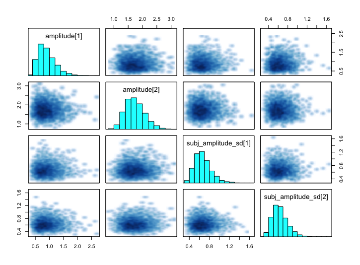
Also, I’ve attached pairs plots for a case in which some parameters are sample well and for a case in which some parameters are not sampled well (exceeding maximum treedepth).
I have a bundle of scripts and data that can reproduce my issues that I can link to (Google Drive of something) if necessary.
You probably don’t want to use Cauchy priors on the length scales of your GP. The priors that allow for length scales shorter than the distances between your data points are kinda nasty I think. Also, Cauchy’s allow for crazy big ones. Try tightening up your length scale priors and see if that helps.
I think the standard recommendation now is to use some sorta zero-avoiding prior for the length scale. The examples in the manual are mostly gamma(4, 4) now, for instance. Check out Section 18.3 in the new (edit: 2.16) manual, and especially the bit “Priors for Gaussian Process Parameters”.
# next line implies subj_volatility ~ cauchy(0,subj_volatility_sd)
noise_subj_volatility[zi] = noise_subj_volatility_sd[zi] * tan(noise_subj_volatility_helper[zi]) ;
Also, is there a reason to not use the cauchy syntax here? I’ve seen this a couple times in the last couple days and I’m curious.
Thanks for the reply. I’ve just noticed that I did not make it clear that the Cauchy is on what I’ve been calling volatility. Mike Lawrence, my rstan mentor of sorts, introduced me to this terminology - its more interpretable to lay audiences. Anyway, volatility is the inverse of the length scale. Therefore, as it stands the prior avoids unreasonably small length scales, but allows for very large length scales.
Ghislain was on the students in the GP summer school and we discussed after my presentation.
My guess was that Cauchy is making the tails too heavy as max treedepth was exceeded often. It didn’t look like zero avoiding prior would be necessary for lengthscales. The model is hierarchical GP instead of simple GP, and I guess that causes some identifiability problems, and would need more thought for the priors at different levels. I recommended posting here to get more eyes to check the model.
Yes, if noise_subj_volatility_helper[zi] is uniform between -pi() / 2 and pi() / 2, then a priori in the unconstrained space, it is logistic, which has fairly reasonable tails. Also, it is a priori independent of noise_subj_volatility_sd[zi]. If you were to make noise_subj_volatility[zi] a primitive parameter with a cauchy(0, noise_subj_volatility_sd[zi] prior, it would have unreasonable tails in the unconstrained space and dependence with noise_subj_volatility_sd[zi], neither of which are helpful for NUTS.
Apologies, I haven’t actually thought that through. Mike recommended the cauchy form initially and I simply know that it reasonably matched my prior beliefs about the hyperparameter.
I’ve played around with using a normal instead of a cauchy
Sigh, my reading comprehension sucks. I got too excited Ye Olde Standard Advice would fix your problems. Inverse normal is definitely gonna be zero avoiding.
Do the treedepth warnings go away once you increase max_treedepth and adapt_delta?
Also, I’ve attached pairs plots for a case in which some parameters are sample well and for a case in which some parameters are not sampled well (exceeding maximum treedepth).
Is is that half the time the chains sample well and half the time they don’t?
Does this model with these priors fit a single subject well? (if that makes sense)? Like if it’s not hierarchical?
I have a bundle of scripts and data that can reproduce my issues that I can link to (Google Drive of something) if necessary.
If it’s not too much work on you, I wouldn’t mind running it and havin’ a look.
Do the treedepth warnings go away once you increase max_treedepth and adapt_delta?
Yes.
Is is that half the time the chains sample well and half the time they don’t?
No. If the max_treedepth and adapt_delta are low then it always samples badly. If the max_treedepth and adapt_delta are sufficiently high then it always samples properly (it just takes a long time).
Does this model with these priors fit a single subject well? (if that makes sense)? Like if it’s not hierarchical?
I can’t remember if I’ve explicitly run that test. I believe I have. Anyway, I would be surprised if the priors don’t. The simulation I’ve conducted with max_treepdepth and adapt_delta set to 15 and 0.99 was very successful - the model captures the true parameters within its 50% or 95% credibility estimates across the board.
Is there a big compelling reason to model the noise in the data as a GP? That seems difficult. Is there a way to get by without this? It’s easier if we can think about noise as iid measurement noise, but if it needs to be complicated so be it :P.
It looks like the GPs are computed across this thing x which is pretty short (length 16). The outputs are labeled with these z_by_f_by_s_pad things that get everything in the right place (I was trying to visualize the meaning of y[si,1:subj_obs[si]] ~ normal(to_vector(z_by_f[si])[z_by_f_by_s_pad[si,1:subj_obs[si]]], ...);.
So the xs in the GPs are meant to represent the distance between places in this periodic signal? Should I be looking at a single time series as the concatenation of a bunch of samples of this GP?
And if this is the case, should the GP be periodic? It seems like x = 1.0 should be related to x = 0.0.
First off, thanks for taking the time to look through this. I really appreciate it.
Your plots are not representative of the data. I’ve added some files to the shared folder in Google Drive. If you turn your attention to the ‘analyzing_GPs’ file you’ll get a better sense for how the raw (simulated) data (‘fake_data_proposal’) are rearranged to facilitate entry into the stan model. Basically, the index structures are created to easily associate particular ‘y’ values wit with unique experimental conditions and subjects. The idea is to minimize the amount of looping required in the stan code.
As for modelled heteroscedasticity, that happens to generally be an important outcome in the field in which I intend to apply this model (in motor control, researchers make explicit predictions about the trial-by-trial variability in the data). There are certain cases where iid error assumptions may be appropriate, but in general it is a valuable model feature for my application case.
I’ve attached some plots of the raw (simulated) data so you know what I’m trying to model:
These GPs look like they’re modeling really flat functions. I’ve had trouble before fitting GPs to flat lines, strangely enough. That’s Ye Olde First Guess, but I’ll take a look at it when I get bored of doin’ other stuff later in the afternoon.
I have to say this has me stumped. I messed around with some more and it seems like, whatever I do, treedepth is exceeded.
I’m going to let it sit for awhile and think about it, but I tried all the obvious things. I put tighter priors that stay away from infinity and zero; I simplified how the hyperpriors worked (made all subjects share a length scale/amplitude, which I think makes sense here); and eventually I actually just made the priors fixed and it’s still having problems (but maybe I just chose bad fixed parameters too…).
It doesn’t seem like there’s anything bad about the model, per se, it’s just difficult to sample haha. Right now I’m blaming the latent GP parameters themselves, but who knows.
I think the next thing to do would be just try modeling a single subject’s mean and variance. I’ll get around to that sometime in the next couple days, but I figured I’d letcha know what I tried. Hope that is at all useful!
If tighter priors don’t help then it’s likely that there is non-identifiability issue with so many components summed without constraints and the same time small step-size required due to the strong dependencies from GP prior.
Thanks again for taking a look through. Yes, I believe one could justify having a single amplitude and volatility parameter for all participant functions. I am surprised that didn’t help sampling in some way. It is actually something I’ve been meaning to try. Anyway, it is nice to hear in a sense that I wasn’t missing something too obvious. Of course, it is too bad that this model can’t be sampled properly in a shorter amount of time as is… That’s what I get for implementing complicated models!
What Aki said reminded me – I also got rid of the group-level GP and that didn’t really help things (so that the only shared bit of the model were the length scales/amplitudes).
It definitely seems like there could be a little bit of nastiness between the GP in the mean and the GP in the standard deviation, considering the exponent is -(x - u)^2 / (2 * sigma^2) (one might try to cancel the other out and create an unidentifiability).