Hi all,
To be able to modify the plot at will I want reproduce the plot obtained with:
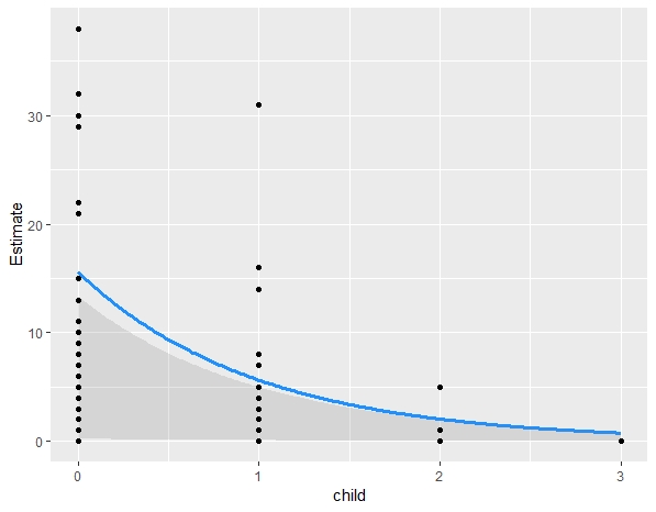
plot(marginal_effects(MODEL_NAME), points=T)
As an example I used the data from
https://stats.idre.ucla.edu/r/dae/zip/
https://stats.idre.ucla.edu/stat/data/fish.csv
deleting a couple of extreme points for plot purposes:
fish<-read.csv(“https://stats.idre.ucla.edu/stat/data/fish.csv”)
fish$camper<-as.factor(fish$camper)
fish<-subset(fish, count!=149 & count!=65)
I ran the following ZERO-INFLATED model
mod_pois_zero = brms::brm(count ~ child + camper +(1| persons),
control = list(adapt_delta = 0.999, max_treedepth = 12),
iter = 6000,
cores = 4,
data = fish,
family = “zero_inflated_poisson”,
file=“mod_pois”)
I wrote the following script to plot estimate and raw data as for marginal_effects:
#extract posterior samples
d<-posterior_samples(mod_pois)
#select the variable(s) you want to plot
d_sub<-d[,c("b_Intercept", "b_child")]
#transform it to a matrix
d_sub1<-as.matrix(d_sub)
# to plot my simulation I have to extract the effect and add them to my original dataset
newdat<-data.frame(b_child = seq(-0,3, by = 0.025))
#if you choose the same length of your database you can add it easily
#put the entire range of your data
#create the matrix you are going to fill
Xmat <-model.matrix(~ b_child, data=newdat)
fitmat<-matrix(ncol=nrow(d), nrow=nrow(newdat))
#Fill the matrix
for(i in 1:nrow(d)) fitmat[,i] <- exp(Xmat%*%d_sub1[i,]) #poisson model
#for(i in 1:nrow(d)) fitmat[,i] <- Xmat%*%d_sub1[i,] #gaussian model
#add the credible interval and fit
newdat$lower<- apply(fitmat,1,quantile, prob=0.025)
newdat$upper<-apply(fitmat, 1, quantile, prob=0.975)
newdat$fit<-apply(fitmat, 1, quantile, prob=0.5)
#newdat$fit<-exp(Xmat%*% fixef(mod_pois)) #fixef does not work in brms
#now you can either merge newdat with your original database or plot them directly
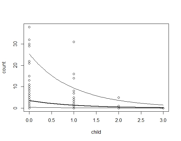
plot(fish$count ~fish$child,
xlab =("b"), ylab = ("a"))
lines(newdat$b_child, newdat$fit, lwd=2)
lines(newdat$b_child, newdat$lower)
lines(newdat$b_child, newdat$upper)
the script works fine for norm and poisson models but the estimates with zero_inflated are wrong.
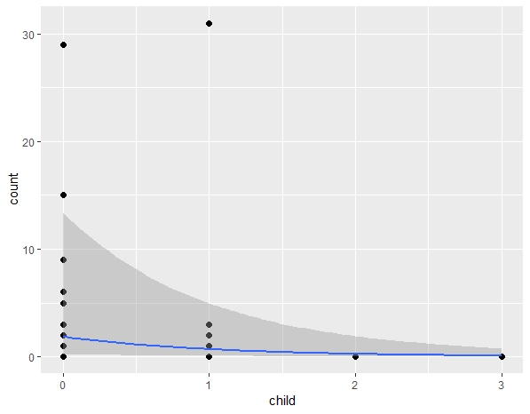
How can I back-transform zero inflated models? clearly exp() is not enough.
Where can I find this information for the rest of the link functions ( e.g. skew normal, etc.)?
On a different note, the default plot plot(marginal_effects(MODEL), points=T) always cut the extreme points, any idea why?
Also if someone has a better strategy to plot raw data and estimates from brms I would be glad to know. Online I could not find any example that I was able to reproduce.
Thanks and best regards