Hi all,
Apologies in advance for the long post - feel free to jump to the Questions section at the end.
Background
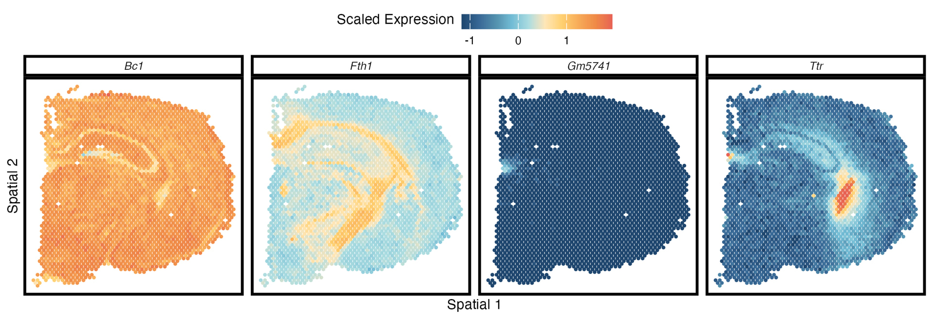
Over the past year or so I’ve been working on developing a hierarchical approximate Gaussian process (GP) model for spatial transcriptomics datasets. The data are composed of an n_s \times n_g counts matrix that has been normalized and scaled, and an n_s \times 2 coordinates matrix that has also been scaled. The subscripts s and g correspond to “spots” (small groups of individual cells) and genes, respectively. The goal of the model is to flexibly & accurately identify genes whose expression exhibits strong spatial dependence i.e., if you visualized their expression on the coordinates you would see distinct patterns such as those shown below. Such genes are called spatially variable genes (SVGs).
Methodology
The math bit
The scaled, normalized expression of gene g at spot i follows a Gaussian likelihood defined like so:
where the mean is defined as:
In the above equation \beta_{0_g} represents the gene-specific intercept, \tau_g is the gene-specific amplitude (or marginal SD) of the GP, \tilde{\phi}(s_i) is the i^{\text{th}} row of the n_s \times k matrix of orthonormal basis functions used to capture the underlying spatial structure, and \alpha_g is the corresponding vector of gene-specific basis function coefficients.
In addition, by default we estimate the j = 1, \dots, k basis functions using the exponentiated quadratic kernel:
where c_j is the j^{\text{th}} centroid obtained after running k-means clustering on the scaled coordinates. The estimated global length-scaled of the GP \hat{\ell} is taken to be the median of the Euclidean distances between the k cluster centroids.
The code bit
All of this is implemented in Stan (with non-centered priors for the gene-specific intercepts and basis function coefficients).
data {
  int<lower=1> M;  // number of spots
  int<lower=1> N;  // number of gene-spot pairs in long dataframe
  int<lower=1> G;  // number of genes
  int<lower=1> k;  // number of basis functions used to approximate GP
  array[N] int<lower=1, upper=M> spot_id;  // unique ID for each spot
  array[N] int<lower=1, upper=G> gene_id;  // unique ID for each gene
  matrix[M, k] phi;  // matrix of QR-decomposed basis functions used to approximate GP
  vector[N] y;  // vector of normalized, scaled gene expression used as response variable
}

parameters {
  real mu_beta0;  // mean for the global intercepts
  real<lower=0> sigma_beta0;  // SD for the global intercepts
  vector[G] z_beta0;  // vector of standard normal RVs for the global intercepts
  real mu_amplitude;  // mean for the amplitude
  real<lower=0> sigma_amplitude;  // SD for the amplitude
  vector<lower=0>[G] amplitude;  // vector of gene-specific amplitudes of the approximate GP
  vector[k] mu_alpha;  // vector of means for the basis function coefficients
  vector<lower=0>[k] sigma_alpha;  // vector of SDs for the basis function coefficients
  matrix[k, G] z_alpha_t;  // standard normal RV for basis function coefficients
  real<lower=0> sigma_y;  // observation noise of response variable
}

transformed parameters {
  vector[G] beta0 = mu_beta0 + sigma_beta0 * z_beta0;
  vector[G] amplitude_sq = square(amplitude);
}

model {
  matrix[k, G] alpha_t;
  alpha_t = rep_matrix(mu_alpha, G) + diag_pre_multiply(sigma_alpha, z_alpha_t);
  matrix[M, G] phi_alpha = phi * alpha_t;
  vector[N] w;
  for (i in 1:N) {
    w[i] = phi_alpha[spot_id[i], gene_id[i]];
  }
  to_vector(z_alpha_t) ~ std_normal();
  z_beta0 ~ std_normal();
  mu_beta0 ~ normal(0, 2);
  sigma_beta0 ~ std_normal();
  mu_amplitude ~ normal(0, 2);
  sigma_amplitude ~ std_normal();
  amplitude ~ lognormal(mu_amplitude, sigma_amplitude);
  mu_alpha ~ normal(0, 2);
  sigma_alpha ~ std_normal();
  sigma_y ~ std_normal();
  y ~ normal(beta0[gene_id] + amplitude_sq[gene_id] .* w, sigma_y);
}
After formatting the spatial transcriptomics data such that it matches the structure of the model, I use cmdstanr to perform the fitting. First, I run a quick optimization to initialize all of the model parameters near their modes, as I’ve seen empirically that this increases convergence speed for the next step - fitting the model using variational inference (VI). Here’s what the full process looks like:
model_init <- mod$optimize(data_list,
                           seed = random.seed,  # defaults to 312
                           init = 0,
                           opencl_ids = opencl_IDs,  # defaults to NULL
                           jacobian = FALSE,
                           iter = mle.iter,  # defaults to 1000
                           algorithm = "lbfgs",
                           history_size = 25L)
fit_vi <- mod$variational(data_list,
                          seed = random.seed,  # defaults to 312
                          init = model_init,
                          algorithm = algorithm,  # defaults to "meanfield"
                          iter =  n.iter,  # defaults to 3000
                          draws = n.draws,  # defaults to 1000
                          opencl_ids = opencl_IDs,  # defaults to NULL
                          elbo_samples = elbo.samples)  # defaults to 150
Finally, I use the posterior package to generate (by default) 1000 draws from the variational posterior of \hat{\tau}_g for every gene g. Taking the mean of the draws gives a point estimate of spatial variability for every gene that can then be used to rank the genes with e.g., the top 1000 genes by estimated amplitude being designated as SVGs.
All of this is implemented in a much more user-friendly manner in my R package bayesVG.
Challenges
- High dimensionality - typically the number of genes n_g \in [2000, 4000]
- Scalability - depending on the technology used the sequence the raw tissue, the number of observations n_s can range from from the thousands (e.g., 10X Visium) to the hundreds of thousands (e.g., 10X Xenium)
- Interpretability - whatever parameter estimate used to rank & select SVGs should have an interpretation grounded in the underlying biology
- Accuracy - the variational posterior might not be a good enough approximation to the true posterior
The last point (accuracy) is the one I’m still working on and am currently concerned about.
Questions
I’ve read a decent amount about how to perform posterior predictive checks (PPCs) for models fit using classical MCMC sampling such as, for example, the official Stan documention and the documentation for the loo package used to perform leave-one-out cross-validation. However, neither resource has examples or information related to models fit using VI.
I also read this great preprint on evaluating the quality of the variational approximation, but I’m not quite sure how to take the concepts there and turn them into working R + Stan code. I know I need to add a generated quantities block to the Stan code, I just don’t know what I need to put there or how to process it after fitting.
Any hints on how to approach this would be greatly appreciated !
-Jack