Partial pooling on ordinal response (cumulative probit)

New question from a newbie who tries to wrangle my brain around cumulative probit models (ordinal responses, in this case a 7-item Likert, coded as 1-7)

I have skewed data (currently 7 respondents, each replying to 6 questions) as per the below:

 # each respondent answers 6 questions on a 7-point Likert (coded as 1-7)
data <- data.frame(
  id=rep(c("A", "B", "C", "D", "E", "F", "G"), each=6),
  gender=c(rep("male", 6*4), rep("female", 6*3)),
  name=rep(c("Q1", "Q2", "Q3", "Q4", "Q5", "Q6"), times=7),
  response=c(rep(6,6), # resp.1, male
             c(rep(7,4), rep(6,2)), # resp.2, male
             rep(7,6), # resp.3, male
             c(7, rep(6,4), 5), # resp.4, male
             rep(7, 6), #resp.5, female
             rep(6, 6), #resp.6, female
             c(7, 6, 6, rep(5,3)) # resp.7, female
             ))
data |> group_by(id, gender, response) |> tally()

When I fit a regular, non-pooled model, things line up to the data quite nicely:

d <- data |> select(response, gender)
formula <- response | thres(6) ~ 1 + gender
priors <- c(prior(normal(-1.068, 1), class = Intercept, coef = 1),
            prior(normal(-0.566, 1), class = Intercept, coef = 2),
            prior(normal(-0.180, 1), class = Intercept, coef = 3),
            prior(normal( 0.180, 1), class = Intercept, coef = 4),
            prior(normal( 0.566, 1), class = Intercept, coef = 5),
            prior(normal( 1.068, 1), class = Intercept, coef = 6),
            prior(normal(0, 1), class = b))
M2 <- brm(
  data = d,
  family = cumulative(probit),
  formula=formula,
  prior = priors,
  backend="cmdstanr",
  cores = 4,
  seed = 1
)
m <- M2

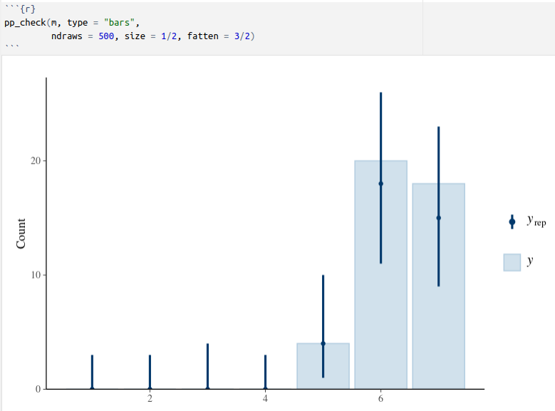
Diagnostics look OK (around 40ish divergent transitions, but the caterpillar plots look OK, etc)
Posterior predictive plots line up to the data:

I modified the plot function from the blog that @Solomon provides here Notes on the Bayesian cumulative probit | A. Solomon Kurz (it has helped me a lot) to fit my data (e.g. I use 7-item Likert):

plot_M2_posterior_mean <- function(m, title) {
  m_male <- m$data |> filter(gender == 'male') |> summarize(m=mean(response)) |> pull()
  m_female  <- m$data |> filter(gender == 'female') |> summarize(m=mean(response)) |> pull()
  # note, the magrittr pipe %>% is needed, because native |> pipe does not handle dot
  as_draws_df(m) %>%
    select(.draw, starts_with("b_")) %>%
    set_names(".draw", str_c("tau[", 1:6, "]"), "beta[1]") %>%
    # insert another copy of the data below
    bind_rows(., .) %>%
    # add the two values for the dummy variable gendermale
    mutate(gendermale = rep(0:1, each = n() / 2)) %>%
    # compute the p_k values conditional on the gender dummy
    mutate(p1 = pnorm(`tau[1]`, mean = 0 + gendermale * `beta[1]`),
           p2 = pnorm(`tau[2]`, mean = 0 + gendermale * `beta[1]`) - pnorm(`tau[1]`, mean = 0 + gendermale * `beta[1]`),
           p3 = pnorm(`tau[3]`, mean = 0 + gendermale * `beta[1]`) - pnorm(`tau[2]`, mean = 0 + gendermale * `beta[1]`),
           p4 = pnorm(`tau[4]`, mean = 0 + gendermale * `beta[1]`) - pnorm(`tau[3]`, mean = 0 + gendermale * `beta[1]`),
           p5 = pnorm(`tau[5]`, mean = 0 + gendermale * `beta[1]`) - pnorm(`tau[4]`, mean = 0 + gendermale * `beta[1]`),
           p6 = pnorm(`tau[6]`, mean = 0 + gendermale * `beta[1]`) - pnorm(`tau[5]`, mean = 0 + gendermale * `beta[1]`),
           p7 = 1 - pnorm(`tau[6]`, mean = 0 + gendermale * `beta[1]`)) %>%
    # wrangle
    pivot_longer(starts_with("p"), values_to = "p") %>%
    mutate(response = str_extract(name, "\\d") %>% as.double()) %>%
    # compute p_k * k
    mutate(`p * response` = p * response) %>% 
    # sum those values within each posterior draw, by the gendermale dummy
    group_by(.draw, gendermale) %>% 
    summarise(mean_response = sum(`p * response`)) %>% 
    mutate(gender = ifelse(gendermale == 0, "female", "male")) %>% 
    
    # the trick with and without fct_rev() helps order the axes, colors, and legend labels
    ggplot(aes(x = mean_response, y = fct_rev(gender), fill = gender)) +
    stat_halfeye(.width = .95) +
    geom_vline(xintercept = m_male, linetype = 2, color = "blue3") +
    geom_vline(xintercept = m_female, linetype = 2, color = "red3") +
    scale_fill_manual(NULL, values = c(alpha("red3", 0.5), alpha("blue3", 0.5))) +
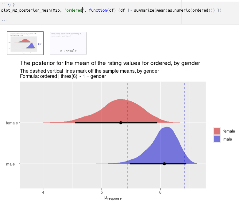
    labs(title = paste0("The posterior for the mean of the rating values for ", title, ", by gender"),
         subtitle = paste("The dashed vertical lines mark off the sample means, by gender\nFormula:", m$formula),
         x = expression(mu[response]),
         y = NULL) +
    theme(axis.text.y = element_text(hjust = 0)) 
}

Using this function seems to show reasonable alignment with the sample mean:

However, I have learned that in order to avoid overfitting, and make the model more generalizable, I should use partial pooling, and in my case I thought that using pooling on respondents as well as on questions might make scientific sense.
Some respondents might have a bad day, or some questions might be vaguely formulated, so it makes sense to pool that information into the overall model.
I am not overly interested in the actual responses for specific respondents, or specific questions, so when I make predictions, I still intended to only use gender as a predictor (plus the intercept of course).
I figured that I could reuse the function above to plot data from the pooled model as well.
From what I understand, the group-level effects (only affecting intercepts, in my case) work like “offsets from the population parameter”, so if I omit them from the calculation, I would get the behaviour of “the average respondent, responding to the average question” (average in the model-sense, not necessarily arithmetic average).

So, also based on Solomons writings, I defined the following model:

d <- data |> select(response, gender, id, name)
formula <- response | thres(6) ~ 1 + gender + (1 | id) + (1 | name)
priors <- c(prior(normal(-1.068, 1), class = Intercept, coef = 1),
            prior(normal(-0.566, 1), class = Intercept, coef = 2),
            prior(normal(-0.180, 1), class = Intercept, coef = 3),
            prior(normal( 0.180, 1), class = Intercept, coef = 4),
            prior(normal( 0.566, 1), class = Intercept, coef = 5),
            prior(normal( 1.068, 1), class = Intercept, coef = 6),
            prior(normal(0, 1), class = b),
            prior(exponential(1), class = sd))
M3 <- brm(
  data = d,
  family = cumulative(probit),
  formula=formula,
  prior = priors,
  backend="cmdstanr",
  cores = 4,
  seed = 1
)
m <- M3

Posterior checks look good, both on population level and grouped by id or name.

When I use the same function as above to plot the mean of the response, I get considerable drift towards the middle of the range:

plot_M2_posterior_mean(m, "response")

At first, I figured that this makes sense. I now use partial pooling, making the mean drift towards the population mean, and individual respondents are less influential.

However, I tested by simulating that I got 40 new rave reviews (all 7, the max response)
This turns the model even more towards the center of the scale, which I find counter-intuitive:

d <- rbind(data |> select(response, gender, id, name), 
           data.frame(response=7, # rave reviews 
                      gender=rep(c("female", "male"), each=120),
                      id=rep(c("100", "101", "102", "103", "104", "105", "106", "107", "108", "109",
                               "1100", "1101", "1102", "1103", "1104", "1105", "1106", "1107", "1108", "1109",
                               "200", "201", "202", "203", "204", "205", "206", "207", "208", "209",
                               "2100", "2101", "2102", "2103", "2104", "2105", "2106", "2107", "2108", "2109"), each=6), # 40 new respondents
                      name=rep(c("Q1", "Q2", "Q3", "Q4", "Q5", "Q6"), times=40)))

plot_M2_posterior_mean(
  brm(
    data = d,
    family = cumulative(probit),
    formula=formula,
    prior = priors,
    backend="cmdstanr",
    cores = 4,
    seed = 1),
  "faked response")

Gives the plot:

Before adding the fake reviews, the pooled model had means close to 5 (whereas the non-pooled model was more optimistic, around 6). After adding 40 new respondents, each replying 7 to every question, the expected mean response decreases to around 4.5

What am I misunderstanding? Or mis-coding?
After all, I adapted the code from the blog of @Solomon as above, and I am quite new to ordinal modeling (as stated before here). Thanks in advance!

  • Operating System: Ubuntu 22.04
  • brms Version: 2.22.0

Hey @epkanol, there’s a lot going on here, so I’ll start with a few points and we’ll go from there.

First, I recommend against naming any data set data, which can make for conflicts with the base data() function. Let’s just call the data d.

Second, your response variable is currently numeric. My impression has always been brm() expects ordered factors for ordinal models. Thus I’ll be saving a version of response as ordered. However, I should note here that I was not able to confirm this with a review of the brms reference manual (link) which I found very surprising, and which makes me wonder if brms has changed some of its behavior in recent versions.

With those in mind, here’s an update of the data.

# Packages
library(tidyverse)
library(brms)
library(tidybayes)

# Make the data
d <- data.frame(
  id = rep(c("A", "B", "C", "D", "E", "F", "G"), each = 6),
  gender = c(rep("male", 6 * 4), rep("female", 6 * 3)),
  # `name` stands for "item"
  name = rep(c("Q1", "Q2", "Q3", "Q4", "Q5", "Q6"), times = 7),
  response = c(rep(6, 6),              # resp.1, male
             c(rep(7, 4), rep(6, 2)),  # resp.2, male
             rep(7, 6),                # resp.3, male
             c(7, rep(6, 4), 5),       # resp.4, male
             rep(7, 6),                # resp.5, female
             rep(6, 6),                # resp.6, female
             c(7, 6, 6, rep(5, 3)) # resp.7, female
             )) |> 
  # Make an ordered factor version of `response`
  mutate(ordered = factor(response, levels = 1:7, ordered = TRUE))

# Make a high-level count of the data
d |> 
  count(gender, ordered, .drop = FALSE) |> 
  pivot_wider(names_from = gender, values_from = n)
# A tibble: 7 Ă— 3
  ordered female  male
  <ord>    <int> <int>
1 1            0     0
2 2            0     0
3 3            0     0
4 4            0     0
5 5            3     1
6 6            8    12
7 7            7    11

Now we’ll fit two models. The first will be your M2 again. The second will be a new model M2b which uses the ordered factor ordered as the response variable, instead.

priors <- c(prior(normal(-1.068, 1), class = Intercept, coef = 1),
            prior(normal(-0.566, 1), class = Intercept, coef = 2),
            prior(normal(-0.180, 1), class = Intercept, coef = 3),
            prior(normal( 0.180, 1), class = Intercept, coef = 4),
            prior(normal( 0.566, 1), class = Intercept, coef = 5),
            prior(normal( 1.068, 1), class = Intercept, coef = 6),
            prior(normal(0, 1), class = b))
M2 <- brm(
  data = d,
  family = cumulative(probit),
  formula = response | thres(6) ~ 1 + gender,
  prior = priors,
  backend = "cmdstanr",
  cores = 4,
  seed = 1
)

M2b <- brm(
  data = d,
  family = cumulative(probit),
  formula = ordered | thres(6) ~ 1 + gender,
  prior = priors,
  backend = "cmdstanr",
  cores = 4,
  seed = 1
)

Check the summaries.

summary(M2)
summary(M2b)
Warning: There were 86 divergent transitions after warmup. Increasing adapt_delta above 0.8 may help. See http://mc-stan.org/misc/warnings.html#divergent-transitions-after-warmup Family: cumulative 
  Links: mu = probit; disc = identity 
Formula: response | thres(6) ~ 1 + gender 
   Data: d (Number of observations: 42) 
  Draws: 4 chains, each with iter = 2000; warmup = 1000; thin = 1;
         total post-warmup draws = 4000

Regression Coefficients:
             Estimate Est.Error l-95% CI u-95% CI Rhat Bulk_ESS Tail_ESS
Intercept[1]    -2.45      0.60    -3.78    -1.41 1.01      313      123
Intercept[2]    -1.87      0.43    -2.76    -1.09 1.00     1860     1080
Intercept[3]    -1.58      0.36    -2.35    -0.91 1.00     2298     2748
Intercept[4]    -1.38      0.33    -2.09    -0.75 1.00     2876     2579
Intercept[5]    -0.81      0.28    -1.36    -0.26 1.01     1368     2281
Intercept[6]     0.46      0.26    -0.05     0.98 1.00     2949     3053
gendermale       0.23      0.32    -0.39     0.87 1.01     2474     1539

Further Distributional Parameters:
     Estimate Est.Error l-95% CI u-95% CI Rhat Bulk_ESS Tail_ESS
disc     1.00      0.00     1.00     1.00   NA       NA       NA

Draws were sampled using sample(hmc). For each parameter, Bulk_ESS
and Tail_ESS are effective sample size measures, and Rhat is the potential
scale reduction factor on split chains (at convergence, Rhat = 1).
 Family: cumulative 
  Links: mu = probit; disc = identity 
Formula: ordered | thres(6) ~ 1 + gender 
   Data: d (Number of observations: 42) 
  Draws: 4 chains, each with iter = 2000; warmup = 1000; thin = 1;
         total post-warmup draws = 4000

Regression Coefficients:
             Estimate Est.Error l-95% CI u-95% CI Rhat Bulk_ESS Tail_ESS
Intercept[1]    -1.24      0.31    -1.85    -0.64 1.00     2595     2456
Intercept[2]     0.22      0.26    -0.31     0.73 1.00     4243     2961
Intercept[3]     1.68      0.34     1.03     2.37 1.00     3978     3489
Intercept[4]     1.88      0.37     1.18     2.64 1.00     4181     3519
Intercept[5]     2.19      0.44     1.39     3.12 1.00     4522     3109
Intercept[6]     2.73      0.59     1.68     4.00 1.00     4467     3423
gendermale       0.27      0.32    -0.36     0.89 1.00     3621     2989

Further Distributional Parameters:
     Estimate Est.Error l-95% CI u-95% CI Rhat Bulk_ESS Tail_ESS
disc     1.00      0.00     1.00     1.00   NA       NA       NA

Draws were sampled using sample(hmc). For each parameter, Bulk_ESS
and Tail_ESS are effective sample size measures, and Rhat is the potential
scale reduction factor on split chains (at convergence, Rhat = 1).

I would not take those warning messages for M2 lightly. Note the very poor ESS diagnostics for the first threshold. Let’s investigate further with trace plots. Usually plot() is fine for this, but this time we’ll make a custom plot by hand.

par_vec <- c(str_c("b_Intercept[", 1:6, "]"), "b_gendermale")

bind_rows(as_draws_df(M2), as_draws_df(M2b)) |> 
  select(starts_with("."), starts_with("b_")) |> 
  mutate(fit = rep(c("M2", "M2b"), each = n() / 2)) |> 
  pivot_longer(cols = starts_with("b_")) |> 
  mutate(name = factor(name, levels = par_vec),
         chain = factor(.chain)) |> 
  
  ggplot(aes(x = .iteration, y = value, color = chain)) +
  geom_line(linewidth = 1/4) +
  scale_color_viridis_d(option = "D", end = 0.8) +
  ylab("posterior") +
  facet_grid(name ~ fit, scales = "free_y")

We have some ugly looking behavior in the chains for M2, the model where we tried modeling the numeric variable response as ordinal. There might be ways around this, but I recommend otherwise and instead fitting the ordinal model to the ordered factor ordered (as in M2b).

Speaking of which, notice two things about the M2b model based on the ordered factor ordered.

  • The trace plots look much better, as do the HMC diagnostics from the summary() output, above.
  • But also notice how radically different the scales of the threshold posteriors are between the two models (indicated by their placement on the y-axis, per row in the trace plot. I found this very surprising at first, but let’s investigate further with pp_check().
pp_check(M2, type = "bars", ndraws = 500, size = 1/2, fatten = 2/3)
pp_check(M2b, type = "bars", ndraws = 500, size = 1/2, fatten = 2/3)

pp_check() rightly indicated the predictions for the unobserved level were on the lower end of the scale for the numeric response in your M2 model. However, for my M2b model that used the ordered factor version of the variable ordered, pp_check() made the predictions for the missing values on the right! I’m not sure what’s going on, but until it’s clear how to properly model unobserved categories in an ordinal model, I wouldn’t proceed. We may need @paul.buerkner to clarify the issue. Once that’s clear, we can then proceede to the other issues in the later part of your post.

1 Like

Thanks a bunch for your help, again!

I did not get your bad ESS values (though they were lower than the rest), and my chains mixed well, nothing that I saw in mcmc_trace (which is what I usually use, being a newbie).

Regression Coefficients:
             Estimate Est.Error l-95% CI u-95% CI Rhat Bulk_ESS Tail_ESS
Intercept[1]    -2.41      0.57    -3.65    -1.43 1.00     1284      852
Intercept[2]    -1.89      0.41    -2.75    -1.13 1.00     2524     1861
Intercept[3]    -1.59      0.36    -2.32    -0.94 1.00     3227     3017
Intercept[4]    -1.40      0.32    -2.06    -0.80 1.00     3127     2468
Intercept[5]    -0.81      0.27    -1.34    -0.26 1.00     3301     2682
Intercept[6]     0.45      0.27    -0.07     0.98 1.00     3165     2631
gendermale       0.21      0.33    -0.43     0.86 1.00     2847     2119

When switching to ordered, I did get the strange reordering that you mentioned, so there is something fishy going on in brms when dealing with ordered levels that are not present in the data.
When I artificially create one row for every ordered category (e.g. by changing the last respondent values to: c(1, 2, 3, 4, rep(5,2)) # resp.7, female, I get literally the same behaviour for both M2 and M2b (they do use the same seed)

Regression Coefficients:
             Estimate Est.Error l-95% CI u-95% CI Rhat Bulk_ESS Tail_ESS
Intercept[1]    -1.76      0.42    -2.66    -1.03 1.00     2516     1780
Intercept[2]    -1.28      0.32    -1.94    -0.67 1.00     4602     3114
Intercept[3]    -0.97      0.29    -1.57    -0.42 1.00     4590     3135
Intercept[4]    -0.73      0.28    -1.29    -0.18 1.00     4588     3205
Intercept[5]    -0.39      0.27    -0.91     0.14 1.00     3939     2498
Intercept[6]     0.74      0.27     0.19     1.26 1.00     3487     3016
gendermale       0.58      0.34    -0.09     1.24 1.00     3316     2353

The bad N_{eff}/N value (around 0.1) also disappears for M2 when adding a starting value of 1

The output for the models (with resp.7 values changed as above) are now identical (but I had to change the plot function a bit to accomodate the change in variable name:

plot_M2_posterior_mean <- function(m, title, sample_mean) {
  m_male <- m$data |> filter(gender == 'male') |> sample_mean()  |> pull()
  m_female  <- m$data |> filter(gender == 'female') |> sample_mean() |> pull()
  # note, the magrittr pipe %>% is needed, because native |> pipe does not handle dot
<rest as before>

With the original data (lacking any 1,2,3 or 4 in the Likert data), the ordered variant breaks down completely. It seems to be confusing levels, making predictions meaningless (as you would not know what the levels meant).
We’ll have to wait what @paul.buerkner says.

Thanks a bunch for keeping the discourse, and trying to explain what goes of for a newbie like me.

I realized that I could reverse the scales, and check how brms handles that as an ordinal factor.
This turns out to work well (less than 10 divergent transitions), and ESS sizes are equal for the numeric and ordered variants
Here are my new variables (I kept the original also, to be able to compare models):

df <- data.frame(
  id=rep(c("A", "B", "C", "D", "E", "F", "G"), each=6),
  gender=c(rep("male", 6*4), rep("female", 6*3)),
  name=rep(c("Q1", "Q2", "Q3", "Q4", "Q5", "Q6"), times=7),
  response=c(rep(6,6), # resp.1, male
             c(rep(7,4), rep(6,2)), # resp.2, male
             rep(7,6), # resp.3, male
             c(7, rep(6,4), 5), # resp.4, male
             rep(7, 6), #resp.5, female
             rep(6, 6), #resp.6, female
             c(7, 6, 6, rep(5,3)) # resp.7, female
             )) |>
  mutate(ordered=factor(response, levels=1:7, ordered=TRUE),
         reversed=8-response) |>
  mutate(revorder=factor(reversed, levels=1:7, ordered=TRUE))

So, reversed is the numeric reversed scale, and revorder is the corresponding ordered factor.
In the data set, there are now 18 “1” scores, 20 “2” scores, and 1 “3” score, and no “4”-“7” scores at all.

This turns out to work well for the ordered rank, both in the non-pooled and the pooled versions:

Pooled version:

Adding 40 rave reviews still forces the expected population mean closer towards the middle of the scale:

Here is the code to reproduce that plot:

formula <- revorder | thres(6) ~ 1 + gender + (1 | id) + (1 | name)
d <- rbind(df |> select(revorder, gender, id, name), 
           data.frame(revorder=1, # rave reviews 
                      gender=rep(c("female", "male"), each=120),
                      id=rep(c("100", "101", "102", "103", "104", "105", "106", "107", "108", "109",
                               "1100", "1101", "1102", "1103", "1104", "1105", "1106", "1107", "1108", "1109",
                               "200", "201", "202", "203", "204", "205", "206", "207", "208", "209",
                               "2100", "2101", "2102", "2103", "2104", "2105", "2106", "2107", "2108", "2109"), each=6), # 40 new respondents
                      name=rep(c("Q1", "Q2", "Q3", "Q4", "Q5", "Q6"), times=40)))

plot_M2_posterior_mean(
  brm(
    data = d,
    family = cumulative(probit),
    formula=formula,
    prior = priors,
    backend="cmdstanr",
    cores = 4,
    seed = 1),
  "faked revorder", 
  function(df) {df |> summarize(mean(as.numeric(revorder))) })

I find this counterintuitive. But I am a newbie on ordinal scales, and are most likely doing some mistakes in code or interpretation.

I still wouldn’t move forward until it is 100% clear how to handle unobserved categories with brms.

Just a few comments -
Divergent transitions should not be ignored. Your inference can’t be trusted when HMC doesn’t properly explore the posterior.
Michael Betancourt recently released an excellent update to his ordinal modeling case study that builds ordinal models from the ground up https://betanalpha.github.io/assets/chapters_html/ordinal_modeling.html
@Solomon In this case study he provides an example of the situation where one has unobserved categories. https://betanalpha.github.io/assets/chapters_html/ordinal_modeling.html#homogeneous-ordinal-probabilities-ii
This can manifest as model degeneracy as seen in the models above, however, the models can be fit provided that a prior model on the cutpoints is informative for all categories. This can be done in a couple of ways that result in an induced-Dirichlet prior on the cutpoints. Either derive the cutpoints from baseline probabilities and put a Dirichlet prior on those probabilities (this is what rstanarm does), or model the cutpoints directly and put an induced-Dirichlet prior model on them. This allows one to place a prior on the cutpoints using domain expertise about the probability for each ordinal category (something far more intuitive than cutpoints for a cumulative distribution function), and it keeps the prior on each cutpoint from overlapping (as is implied by the normal priors in your example, although maybe this is somehow handled behind the scenes in brms by an ordered type in Stan, not sure).

Anyway, we can fit a Stan model to @epkanol original data with the unobserved categories without any divergent transitions or ESS warnings.

library(rstan)

d1 <- data.frame(
  id=rep(c("A", "B", "C", "D", "E", "F", "G"), each=6),
  gender=c(rep("male", 6*4), rep("female", 6*3)),
  name=rep(c("Q1", "Q2", "Q3", "Q4", "Q5", "Q6"), times=7),
  response=c(rep(6,6), # resp.1, male
             c(rep(7,4), rep(6,2)), # resp.2, male
             rep(7,6), # resp.3, male
             c(7, rep(6,4), 5), # resp.4, male
             rep(7, 6), #resp.5, female
             rep(6, 6), #resp.6, female
             c(7, 6, 6, rep(5,3)) # resp.7, female
             ))

Now let’s view some prior predictive checks for the induced-Dirichlet prior model. Here we will derive the cutpoints from baseline probabilities rather than fooling with the Jacobian correction and modeling cutpoints directly.
For example, we can look at the prior pushforward for a Dirichlet with uniform probabilities on the ordinal outcome scale using Stan’s fixed parameter algorthim and generated quantities block and some plotting. A Dirichlet with alpha equal to a vector of ones.

#View an induced-Dirichlet prior model with uniform probabilities over the categories
stan_data <- list(N = 1000, ncut = 6, alpha = c(1,1,1,1,1,1,1))

stan_model <- "
functions {
  vector make_cutpoints(vector probabilities, int ncuts) {
    vector[ncuts] cutpoints;
    real running_sum = 0;
      for (n in 1:ncuts) {
        running_sum += probabilities[n];
        cutpoints[n] = inv_Phi(running_sum);
      }
    return cutpoints;
  }
}
data {
  int<lower=1> N;
  int ncut;
  vector[ncut+1] alpha;
}
generated quantities {
  vector[ncut + 1] pi;
  vector[ncut] cutpoints;
  vector[N] pred_y;
    pi = dirichlet_rng(alpha);
    cutpoints = make_cutpoints(pi, ncut);
    for (n in 1:N) {
      pred_y[n] = ordered_probit_rng(0, cutpoints);
    }
}
"

fit <- stan(model_code = stan_model, data = stan_data,
             chains = 1, iter = 1000, algorithm="Fixed_param")

pred_y <- extract(fit)$pred_y

c_light <- c("#eff3ff")
c_light_highlight <- c("#c6dbef")
c_mid <- c("#9ecae1")
c_mid_highlight <- c("#6baed6")
c_dark <- c("#3182bd")
c_dark_highlight <- c("#08519c")

B <- stan_data$ncut + 1

idx <- rep(1:B, each=2)
x <- sapply(1:length(idx), function(b) if(b %% 2 == 0) idx[b] + 0.5 else idx[b] - 0.5)

pred_counts <- sapply(1:500, function(n) 
                      hist(pred_y[n,], breaks=(1:(B + 1)) - 0.5, plot=FALSE)$counts)
pred_counts_prob <- pred_counts / 1000
probs = c(0.1, 0.2, 0.3, 0.4, 0.5, 0.6, 0.7, 0.8, 0.9)
cred <- sapply(1:B, function(b) quantile(pred_counts_prob[b,], probs=probs))
pad_cred <- do.call(cbind, lapply(idx, function(n) cred[1:9,n]))

plot(1, type="n", main="Prior Predictive Distribution for pred_y",
     xlim=c(0.5, B + 0.5), xlab="pred_y",
     ylim=c(0, 1), ylab="Probability")

polygon(c(x, rev(x)), c(pad_cred[1,], rev(pad_cred[9,])),
        col = c_light, border = NA)
polygon(c(x, rev(x)), c(pad_cred[2,], rev(pad_cred[8,])),
        col = c_light_highlight, border = NA)
polygon(c(x, rev(x)), c(pad_cred[3,], rev(pad_cred[7,])),
        col = c_mid, border = NA)
polygon(c(x, rev(x)), c(pad_cred[4,], rev(pad_cred[6,])),
        col = c_mid_highlight, border = NA)
lines(x, pad_cred[5,], col=c_dark, lwd=2)

As we can see, the induced-Dirichlet(1,1,1,1,1,1,1) prior model pushes forward to uniform probability over the Likert categories.
If we had domain expertise regarding this, we might use something more informative.

We can now try to fit an ordered probit model to your data with unobserved categories using the induced-Dirichlet prior above for the cutpoints.

d1$gender_b <- 0
d1$gender_b <- ifelse(d1$gender=="female", 1, d1$gender_b)

stan_data <- list(N = length(d1$response), ncut = 6, likert = as.integer(d1$response), gender = d1$gender_b)

stan_model <- "
functions {
  vector make_cutpoints(vector probabilities, int ncuts) {
    vector[ncuts] cutpoints;
    real running_sum = 0;
      for (n in 1:ncuts) {
        running_sum += probabilities[n];
        cutpoints[n] = inv_Phi(running_sum);
      }
    return cutpoints;
  }
}
data {
  int<lower=1> N;
  int likert[N];
  vector[N] gender;
  int ncut;
}
parameters {
  simplex[ncut + 1] pi;
  real alpha;
  real beta;
}
transformed parameters {
  vector[ncut] cutpoints = make_cutpoints(pi, ncut);
}
model {
  // prior
  pi ~ dirichlet(rep_vector(1, ncut + 1));
  alpha ~ normal(0, 5);
  beta ~ normal(0, 5);
  // likelihood
  likert ~ ordered_probit(alpha + beta * gender, cutpoints);
}
generated quantities {
  vector[N] pred_y;
    for (n in 1:N) {
      pred_y[n] = ordered_probit_rng(alpha + beta * gender[n], cutpoints);
    }
}
"

fit_mod <- stan(model_code = stan_model, data = stan_data,
             chains = 4, iter = 2000, cores = 4)

Happily the model fits fine with no diagnostic warnings (at least in the random seed I used, but I don’t suspect any problems). There are no divergent transitions (or any other warning).

Now we can do a retrodictive check to see how well our model fits.

pred_y <- extract(fit_mod)$pred_y

c_light <- c("#eff3ff")
c_light_highlight <- c("#c6dbef")
c_mid <- c("#9ecae1")
c_mid_highlight <- c("#6baed6")
c_dark <- c("#3182bd")
c_dark_highlight <- c("#08519c")

B <- stan_data$ncut + 1

idx <- rep(1:B, each=2)
x <- sapply(1:length(idx), function(b) if(b %% 2 == 0) idx[b] + 0.5 else idx[b] - 0.5)

obs_counts <- hist(stan_data$likert, breaks=(1:(B + 1)) - 0.5, plot=FALSE)$counts
pad_obs_counts <- sapply(idx, function(n) obs_counts[n])

pred_counts <- sapply(1:1000, function(n) 
                      hist(pred_y[n,], breaks=(1:(B + 1)) - 0.5, plot=FALSE)$counts)
probs = c(0.1, 0.2, 0.3, 0.4, 0.5, 0.6, 0.7, 0.8, 0.9)
cred <- sapply(1:B, function(b) quantile(pred_counts[b,], probs=probs))
pad_cred <- do.call(cbind, lapply(idx, function(n) cred[1:9,n]))

plot(1, type="n", main="Posterior Predictive Distribution for pred_y",
     xlim=c(0.5, B + 0.5), xlab="pred_y",
     ylim=c(0, max(c(obs_counts, cred[9,]))), ylab="")

polygon(c(x, rev(x)), c(pad_cred[1,], rev(pad_cred[9,])),
        col = c_light, border = NA)
polygon(c(x, rev(x)), c(pad_cred[2,], rev(pad_cred[8,])),
        col = c_light_highlight, border = NA)
polygon(c(x, rev(x)), c(pad_cred[3,], rev(pad_cred[7,])),
        col = c_mid, border = NA)
polygon(c(x, rev(x)), c(pad_cred[4,], rev(pad_cred[6,])),
        col = c_mid_highlight, border = NA)
lines(x, pad_cred[5,], col=c_dark, lwd=2)

lines(x, pad_obs_counts, col="white", lty=1, lw=2.5)
lines(x, pad_obs_counts, col="black", lty=1, lw=2)


Not too shaby!

1 Like