I’m trying to account for some quite extensive overdispersion in my data by modelling the residual variance via a varying intercept for each observation:
m0 <- brm(new_songs ~ 1 + (1|obs), data=df, family=poisson(),
          chains=4, cores = 4, iter = 4000, warmup = 1000)
Converge and mixing is good, but the Pareto k diagnostics are really bad:
Computed from 12000 by 85 log-likelihood matrix

         Estimate   SE
elpd_loo   -245.7 12.0
p_loo        65.7  1.8
looic       491.5 23.9
------
Monte Carlo SE of elpd_loo is NA.

Pareto k diagnostic values:
                         Count Pct.    Min. n_eff
(-Inf, 0.5]   (good)      0     0.0%   <NA>
 (0.5, 0.7]   (ok)        9    10.6%   182
   (0.7, 1]   (bad)      70    82.4%   23
   (1, Inf)   (very bad)  6     7.1%   9
When modelling using a negative binomial, however, all is good, though looic is a bit higher:
         Estimate   SE
elpd_loo   -351.6 20.7
p_loo         3.1  1.2
looic       703.2 41.3
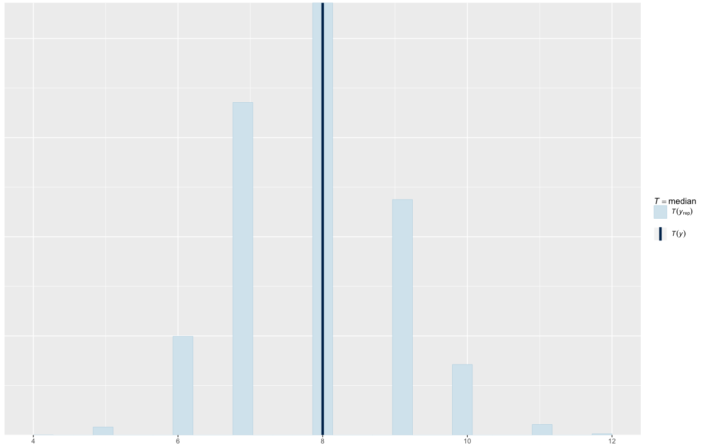
Yet, when looking at the different pp_checks, the poisson model seems to be doing quite OK (see the attached images).
So my question is: should I be worried about the pareto diagnostics (I probably should), or does anyone have a suggestion about how to improve them?

- Operating System: MacOS 10.14.6
- brms Version: brms_2.10.1