Offset multiplier initialization

[bbbales2]

@jsocolar pointed out that if you initialize an offset-multiplier style non-centered parameters to a really small value you get problems sampling. @jsocolar’s example showed the same problems for me, but when I tried to duplicate it with a manual offset-multiplier implementation, I did not get the problem.

It seems like something not-so-good is going on here.

Here is the offset-multiplier model

parameters{
  real<lower = 0> sigma;
  real<multiplier=sigma> x;
}
model{
  sigma ~ std_normal();
  x ~ normal(0, sigma);
}

Here is the manual offset-multiplier model:

parameters{
  real<lower = 0> sigma;
  real x_raw;
}
transformed parameters {
  real x = x_raw * sigma;
}
model{
  sigma ~ std_normal();
  x ~ normal(0, sigma);
  target += log(sigma);
}

Code to run them is

library(tidyverse)
library(cmdstanr)

mod1 = cmdstan_model("mod1.stan")
inits_chain_1 = list(sigma = 1e-20)
fit1 = mod1$sample(chains = 1, init = list(inits_chain_1), iter_sampling = 1000)
fit1$summary()

mod2 = cmdstan_model("mod2.stan")
fit2 = mod2$sample(chains = 1, init = list(inits_chain_1), iter_sampling = 1000)
fit2$summary()

You get output like this for the build-in offset-multiplier:

> fit1$summary()
# A tibble: 3 x 10
  variable      mean    median    sd   mad        q5       q95  rhat ess_bulk
  <chr>        <dbl>     <dbl> <dbl> <dbl>     <dbl>     <dbl> <dbl>    <dbl>
1 lp__     -9.01e+38 -9.01e+38     0     0 -9.01e+38 -9.01e+38    NA       NA
2 sigma     3.12e-20  3.12e-20     0     0  3.12e-20  3.12e-20    NA       NA
3 x        -1.33e+ 0 -1.33e+ 0     0     0 -1.33e+ 0 -1.33e+ 0    NA       NA
# … with 1 more variable: ess_tail <dbl>

And the output with a custom offset-multiplier looks like:

> fit2$summary()
# A tibble: 4 x 10
  variable     mean  median    sd   mad      q5    q95  rhat ess_bulk ess_tail
  <chr>       <dbl>   <dbl> <dbl> <dbl>   <dbl>  <dbl> <dbl>    <dbl>    <dbl>
1 lp__     -1.57    -1.24   0.987 0.761 -3.64   -0.563  1.00     292.     430.
2 sigma     0.821    0.703  0.594 0.591  0.0667  2.02   1.00     437.     366.
3 x_raw     0.0115   0.0396 0.983 1.01  -1.64    1.59   1.00     523.     660.
4 x         0.00698  0.0104 0.967 0.547 -1.66    1.51   1.00     492.     503.

This is pretty repeatable that the custom code doesn’t have a problem with inits but the built in does.

I’m not quite sure where the problem is or what the difference is – posting here if someone knows. @jsocolar said this was happening in a realistic setting (and so figuring out it was a problem probably wasn’t fun or easy and so it’d be nice to fix this if it is fixable or at least know what is the difference)

[rok_cesnovar]

Not sure it helps, but the generated C++ for the first case:

local_scalar_t__ sigma;
sigma = DUMMY_VAR__;
      
sigma = in__.scalar();
if (jacobian__) {
    sigma = stan::math::lb_constrain(sigma, 0, lp__);
} else {
    sigma = stan::math::lb_constrain(sigma, 0);
}
local_scalar_t__ x;
x = DUMMY_VAR__;

x = in__.scalar();
if (jacobian__) {
    x = stan::math::offset_multiplier_constrain(x, 0, sigma, lp__);
} else {
    x = stan::math::offset_multiplier_constrain(x, 0, sigma);
}
{
    lp_accum__.add(std_normal_lpdf<propto__>(sigma));
    lp_accum__.add(normal_lpdf<propto__>(x, 0, sigma));
}

and for the second case:

local_scalar_t__ sigma;
sigma = DUMMY_VAR__;

sigma = in__.scalar();
if (jacobian__) {
  sigma = stan::math::lb_constrain(sigma, 0, lp__);
} else {
  sigma = stan::math::lb_constrain(sigma, 0);
}
local_scalar_t__ x_raw;
x_raw = DUMMY_VAR__;

x_raw = in__.scalar();
local_scalar_t__ x;
x = DUMMY_VAR__;

x = (x_raw * sigma);
{
  lp_accum__.add(std_normal_lpdf<propto__>(sigma));
  lp_accum__.add(normal_lpdf<propto__>(x, 0, sigma));
  lp_accum__.add(stan::math::log(sigma));
}

[bbbales2]

Thanks and this is the offset multiplier code: math/offset_multiplier_constrain.hpp at develop · stan-dev/math · GitHub

Not sure where something is going off the rails. Probably the way to debug this is looking at differences in gradients of those two blocks of C++ tho.

(Edit: to be clear not asking you to check the C++ or anything unless you really want to – the point of the post is to know if anyone else has seen this/knows what is happening before digging in)

[jsocolar]

Just to mention that I think the settings where I’ve seen this happen with “real models” involve initializations far from the typical set where gradients are really weak, and so (with nontrivial probability) chains manage to wander down to absurdly low standard deviations during the initial exploration… and (sinister voice) once they go in, they never come out.

I’ve got a model on simulated data where this was happening as frequently as approximately 1 in 4 chains. Even when chains worked, during the first few iterations this model threw a surprising number of warnings about “multiplier is zero but must be positive” and “current metropolis proposal is about to be rejected” (sorry I don’t have the actual warning text in front of me). Switching to the “old” noncentered parameterization squashed all these warnings as well as the sticky-boundary issue.

[Lu.Zhang]

I agree with @jsocolar that initialization being far from the high probability region could be the problem. The following plot shows the density plot of the offset-multiplier model. The blue and black region has log-density greater than -15. We can see from the plot that the initials will be far from the high probability region when initializing sigma at a very small value.

On the other hand, the high probability region of the manual offset-multiplier has a much better shape. The following plot shows the log-density of the manual offset-multiplier, where the blue and black region has log-density greater than -10.

The weird shape of the high probability region is probably caused by the singularity of the log-density \log p(x, \sigma) of the offset-multiplier model at \sigma = 0 , where \log p(x, \sigma) \propto -0.5 \sigma^2 - log(\sigma) - 0.5 x^2/\sigma^2. While the manual offset-multiplier model whose log-density follows \log p(x_{raw}, \sigma) \propto -0.5 \sigma^2 - 0.5 x_{raw}^2 does not have this problem.

[bbbales2]

Oh wait, when I read this issue a couple days ago I thought these were two different models, but now that I look closer I really think these should be exactly the same two log-densities.

This code from the built-in offset-multiplier (jacobian should be true when we’re doing HMC):

x = in__.scalar();
if (jacobian__) {
    x = stan::math::offset_multiplier_constrain(x, 0, sigma, lp__);
} else {
    x = stan::math::offset_multiplier_constrain(x, 0, sigma);
}
...
lp_accum__.add(lp__) // this happens later in the code

Should be equivalent to:

x = (x_raw * sigma);
...
lp_accum__.add(stan::math::log(sigma));

So I really think these should be the same log densities? I’m confused. Also a lot of the offset_multiplier code and whatnot changed in the last few months so maybe some autodiff got improved in develop. I am curious if this would happen there.

[bbbales2]

@Lu.Zhang

While the manual offset-multiplier model whose log-density follows

I think that density is the one you’d get from a regular non-centered parameterization. Neither of the models in the first post are the regular non-centered parameterization (this is what I missed a couple days ago when I read it).

One of these is offset multiplier and the other should be equivalent to offset multiplier :/.

[Lu.Zhang]

Sorry I am a little bit confused. Isn’t it correct that Stan samples in the unconstrained space of (x, sigma) for the offset-multiplier model, and Stan samples in the unconstrained space of (x_raw, sigma) for the manual offset-multiplier model? The x-axis of the two density plots I gave are different. By the way, I just found that I missed the lower bound of sigma, so I updated the log-density plots in my last post.

[bbbales2]

Ooooo, I think you’re right it is initialization. Underlying they are both exposed to the sampler as x_raw. However, when things are initialized they are initialized on the scale you see, which in the first model is x (not the x_raw scale). In the second model things are indeed initialized on x_raw. Not sure that is actually the problem, but could test that by supplying manual inits.

For more on why both models have an x_raw, what the offset multiplier thing does behind the scenes in sample on an x_raw to avoid that by doing a change of variables transformation from an x_raw to x that should mimic what the second model does.

That’s mostly baked into:

x = stan::math::offset_multiplier_constrain(x, 0, sigma, lp__);

There is the x on the input but that is different than the x on the output (the input should be equivalent to x_raw).

[Lu.Zhang]

@bbbales2

For more on why both models have an x_raw, what the offset multiplier thing does behind the scenes in sample on an x_raw to avoid that by doing a change of variables transformation from an x_raw to x that should mimic what the second model does.

That’s mostly baked into:

x = stan::math::offset_multiplier_constrain(x, 0, sigma, lp__);

I see, that is interesting! Thank you so much!

[bbbales2]

@bbbales2

when things are initialized they are initialized on the scale you see

Wait, I say that with such confidence but it isn’t true lol. Nevermind whoops.

[bbbales2]

(Randomly initialized things are initialized on the unconstrained scale)

[martinmodrak]

Wow, that looks weird.

If that helps anybody, I tried building a Stan model that should match all of the operations and their order as in the offset-multiplier (mod1) and it still does not match the (bad) results in mod1:

mod3.stan:

parameters{
  real<lower = 0> sigma;
  real x_raw;
}
transformed parameters {
}
model{
  real x;
  target += log(sigma);
  x = fma(sigma, x_raw, 0);
  sigma ~ std_normal();
  x ~ normal(0, sigma);
}

So the only remaining difference IMHO is that in mod1 the constraining transform overwrites the x local variable while in mod3 we create a new local variable to hold the result… Which should not matter much?

BTW, I’ve always found the offset-multiplier way of doing stuff confusing as a) it requires me to use sigma at two potentially distant places in the code, increasing risk I will change one but not the other in the future and b) I always have to think hard whether the multiplier is from unconstrained-to-constrained or the other way around. In fact, it seems our own manual has it the wrong way: 10.5 Affinely transformed scalar | Stan Reference Manual (e.g. note that the math there would imply that the log-jacobian is -log(sigma) but Stan’s internal code and comparing with logic of the lower bound both give +log(sigma)) EDIT: I filed a docs issue for this: Docs for affinely transformed scalar do not match implementation · Issue #356 · stan-dev/docs · GitHub

In addition the offset-multiplier logic (both manual and controled by Stan) adds unnecessary operations to the model: log(sigma) is added in the Jacobian correction, only to be subtracted in x ~ normal(0, sigma), with a penalty for both performance and numerical precision, so I think the best way to code non-centering is the IMHO simpler:

parameters{
  real<lower = 0> sigma;
  real x_raw;
}
transformed parameters {
  real x = x_raw * sigma;
}
model{
  sigma ~ std_normal();
  x_raw ~ std_normal();
}

[Lu.Zhang]

Hmm~ I still suspect that the way of generating initials of the two models are different.
If you check the first several samples of x and \sigma for the two models

mod1 = cmdstan_model("mod1.stan")
inits_chain_1 = list(sigma = 1e-7)
fit1 = mod1$sample(chains = 1, init = list(inits_chain_1), 
               iter_sampling = 1000, save_warmup = TRUE)
draws <- fit1$draws(inc_warmup = TRUE)
rbind(draws[1:6,,"x"], draws[1:6,,"sigma"])

mod2 = cmdstan_model("mod2.stan")
fit2 = mod2$sample(chains = 1, init = list(inits_chain_1), 
                   iter_sampling = 1000, save_warmup = TRUE)
draws2 <- fit2$draws(inc_warmup = TRUE)
rbind(draws2[1:6,,"x"], draws2[1:6,,"sigma"])

you will get output like this:

> rbind(draws[1:6,,"x"], draws[1:6,,"sigma"])
          [,1]      [,2]         [,3]         [,4]         [,5]         [,6]
[1,] 0.2110230 0.2110230 -1.30120e-02 -7.56263e-03 -1.14654e-02 -1.61252e-02
[2,] 0.0000001 0.0000001  1.38811e-07  8.30654e-08  1.32924e-07  2.14542e-07
> rbind(draws2[1:6,,"x"], draws2[1:6,,"sigma"])
            [,1]        [,2]        [,3]         [,4]        [,5]        [,6]
[1,] 2.27659e-08 -8.2056e-08 6.52913e-06 -6.68192e-06 0.000232000 0.000181418
[2,] 1.00000e-07  4.5713e-07 5.38727e-06  5.36030e-06 0.000327161 0.003488220

If both models initialize on the unconstrained space of x_{raw} and \sigma, why the scale of x are so different for the two models.

[Funko_Unko]

In case anyone wants to get confused a bit more, here’s a traceplot of the first 200 warmup iterations for a single chain and mod1 and mod2 with a fixed seed but unspecified inits:

Edit with further info:

• Any common seed without inits yields a picture as above
• Specifying only sigma or only x and x_raw as inits yields different initial points and initial traces (as for @Lu.Zhang)
• Specifying sigma and x==x_raw/sigma again yields the same inits and slowly diverging traces.

[Funko_Unko]

Also, @martinmodrak wins a prize:

The other formulations start to do very weird things around sigma==1e-10:

Another edit with further info:

unit corresponds to

@martinmodrak

parameters{
  real<lower = 0> sigma;
  real x_raw;
}
transformed parameters {
  real x = x_raw * sigma;
}
model{
  sigma ~ std_normal();
  x_raw ~ std_normal();
}

Final edit:

left vs right: initialize only sigma vs initialize sigma and x/x_raw
top to bottom: sigma from 1e-20 to 1e-4
colors: models
lines: traceplots in the sigma,|x| plane

black lines: common initial values (if applicable)

Summary:

The manual version only appeared better because the initial points were not the same if only sigma was specified. Actually, it’s not really better than the offset-multiplier version. The reason appears to be numerical, as @martinmodrak’s version works fine for all (tested) values of sigma.

[Dalton]

Coming in 4 years later to chime in that I recently ran into this issue in wild when attempting to fit a logit-normal hierarchical binomial model even with relatively a zero-avoiding prior for sigma. I’m able to achieve convergence by either setting a very small non-zero lower bound on sigma (1e-10) or by switching to a manual non-centered form. But with a lower bound of zero and the affine transform, this model pretty reliably fails.

Here is a reproducible and realistic example of this behavior:

data {
  int<lower = 0>  I;
  array[I] int    N, y;
  real<lower = 0> sigma_lower_bound;
}

parameters {
  real                                     mu;
  real<lower = sigma_lower_bound>          sigma;
  vector<offset=mu, multiplier=sigma>[I]   logit_p;
  // vector[I]                             logit_p_raw;
}

transformed parameters{
  // vector[I] logit_p = mu + logit_p_raw * sigma;
}

model{
  mu      ~ student_t(3, 0, 2.5);
  sigma   ~ loglogistic(1, 4);
  logit_p ~ normal(mu, sigma);
  // logit_p_raw ~ std_normal();
  
  y ~ binomial_logit(N, logit_p);
}

In R:

library(cmdstanr)
library(bayesplot)

I = 1000
p = plogis(rnorm(I, mean = 0.69, sd = 0.5))
N = rpois(I, rgamma(I, 20, 1))
y = rbinom(I, N, p)

binom_hier <- cmdstan_model("binomial_hier.stan")

binom_hier_fit <- binom_hier$sample(data = list(I = I, 
                                                N = N, 
                                                y = y, 
                                                sigma_lower_bound = 0),
                                  chains = 4,
                                  parallel_chains = 4,
                                  refresh = 100,
                                  iter_warmup = 500,
                                  iter_sampling = 500,
                                  save_warmup = T)

Here is the result from running this model:

In this example, the initial values weren’t all that close to the boundary. Chain 1 was 1.3, Chain 2 0.5, Chain 3 0.31 and Chain 4: 1.4. By iteration 5 Chain 2&3 go down to 1e-16 and never recover, but Chain 4 briefly flirts with 1e-10 before bouncing back. It’s like an event horizon down there somewhere.

[Bob_Carpenter]

@bbbales2

However, when things are initialized they are initialized on the scale you see

Other than rejecting for 0 values, you should be able to exactly duplicate behavior between the two approaches if you use your own custom initialization.

The declaration

real<offset=mu, multiplier=sigma> alpha;

means that the “constrained” variable alpha is transformed to the “unconstrained” value (alpha - mu) / sigma. This means that Stan’s default uniform random initialization, which is generically \text{uniform}(-2, 2) in unconstrained space, becomes uniform on (\mu - 2 \sigma, \mu + 2\sigma) in the constrained space where the model is defined. If you manually initialize this way, the behavior should match.

@Dalton

Here is a reproducible and realistic example

This is just one model, so I assume you want us to edit it in the obvious way for the comparison (a reproducible example would require two separate models so they could be compared).

The two models are not equivalent because of the initialization.

P.S. If you have a problem where a lower bound on a scale like sigma feels like a solution, it’s signaling a bigger problem with your model that the lower bound is just sweeping under the carpet (almost always that the data’s consistent with zero variance). If you really want to keep things away from zero, the loglogistic should do that on its own as the density goes to zero as the value goes to zero.

Unless you really think your mu values could be relatively large, you don’t need a wide-tailed distribution like Student-t with 3 degrees of freedom in the prior. Your 99% intervals are (-15, 15) and the 99.9% are (-30, 30), but the tail goes out into values like 100 not being unreasonable. If -30 isn’t a reasonable value, that prior’s too wide. This can wind up causing a problem with fits if you don’t have much data. If you have a ton of data, it should be fine.

[Dalton]

P.S. If you have a problem where a lower bound on a scale like sigma feels like a solution, it’s signaling a bigger problem with your model that the lower bound is just sweeping under the carpet (almost always that the data’s consistent with zero variance). If you really want to keep things away from zero, the loglogistic should do that on its own as the density goes to zero as the value goes to zero.

But the data aren’t consistent with zero variance. It was simulated with non-zero variance. I just reran the model using I = 500, and 8 chains. One got stuck (another flirted with disaster in warm-up and recovered). The lp__ for the chain that got stuck at zero is a lot lower than for the other 7 chains.

Using glm() in R on that same data tell me that the dispersion parameter is 2.

Other than rejecting for 0 values, you should be able to exactly duplicate behavior between the two approaches if you use your own custom initialization.

I’m not convinced this is the initial values, because in the example I posted yesterday, the first iteration values for sigma were all reasonably far from zero. Now I know these aren’t the randomly generated initial values however. So I’m currently working on finding a set that will reproduce this behavior exactly. From trial and error, I can say with the logit-normal hierarchical model, it seems like I’m more likely to run into this issue when I increase the number of draws from the hyperparameter (that is increase I). So maybe the issue is one of the unconstrained logit_phi[i] values being initialized in a way that doesn’t play nicely with the unconstrained sigma and mu values? I’ll see if I can play around and find some initial values that reliably reproduce this.

[Dalton]

Okay, so reporting back in with perhaps stronger evidence of something funky happening with the affine transform in this logit-normal hierarchical model. And while it does seem to have something to do with initial values, it doesn’t appear to be anything in particular about low initial values for sigma.

As suggested I am comparing two “identical” models fit to the same data with the same initial values and the same seed.

As @Bob_Carpenter suggested here are two separate scripts:
binomial_hier_affine.stan

data {
  int<lower = 0>  I;
  array[I] int    N, y;
}
parameters {
  real                                     mu;
  real<lower = 0>                          sigma;
  vector<offset=mu, multiplier=sigma>[I]   logit_p;
}
model{
  mu      ~ student_t(3, 0, 2.5);
  sigma   ~ loglogistic(1, 4);
  logit_p ~ normal(mu, sigma);

  y ~ binomial_logit(N, logit_p);
}

and
binomial_hier_raw.stan

data {
  int<lower = 0>  I;
  array[I] int    N, y;
}
parameters {
  real                     mu;
  real<lower = 0>          sigma;
  vector[I]                logit_p_raw;
}
transformed parameters{
  vector[I] logit_p = mu + logit_p_raw * sigma;
}
model{
  mu      ~ student_t(3, 0, 2.5);
  sigma   ~ loglogistic(1, 4);
  logit_p_raw ~ std_normal();
  
  y ~ binomial_logit(N, logit_p);
}

In R we simulate overdispersed binomial data like so:

I = 500
p = plogis(rnorm(I, mean = 0.69, sd = 0.5))
N = rpois(I, rgamma(I, 20, 1))
y = rbinom(I, N, p)
x = rbinom(I, N, 0.69)

summary(glm(cbind(y, N-y) ~ NULL, family = "quasibinomial"))

We can see that the data are consistent with extrabinomial variation by checking with glm()

(Dispersion parameter for quasibinomial family taken to be 1.935123)

Here is function to generate initial values ensuring that the both models receive the same initial values for both sigma and logit_p/logit_p_raw parameters

init_binom <- function(mu_in, logit_p_raw_in, sigma_in, rand = T){
  inits = list()
  for (i in 1:length(sigma_in)){
    if(rand){
      logit_p_raw = runif(length(logit_p_raw_in[,1]), -2, 2)
      sigma_in = exp(runif(1, -2, 2))
      mu_in = runif(1, -2, 2)
      inits[[i]] = list(mu = mu_in, sigma = sigma_in, 
                        logit_p = mu_in + logit_p_raw*sigma_in,
                        logit_p_raw = logit_p_raw)
    } else{
      logit_p_raw = logit_p_raw_in
      inits[[i]] = list(mu = mu_in[i], sigma = sigma_in[i], 
                        logit_p = mu_in[i] + logit_p_raw[,i]*sigma_in[i],
                        logit_p_raw = logit_p_raw[,i])
    }
  }
  return(inits)
}

And some initial values tests, one deliberately checking low initial values of sigma and holding other parameters fixed and the other checking with random values that I think should be similar to how Stan generates them.

mu_init = rep(0.69, 8)
sigma_chain = c(1e-21, 1e-15, 1e-10, 1e-6, 1e-3, 0.01, 0.1, 1)
logit_p_raw_init = matrix(nrow = I, ncol = 8)
for (i in 1:8)
  logit_p_raw_init[,i] = rep((0.7 - mu_init[i]) / sigma_chain[i], I)

set.seed(125)

inits_nonrandom = init_binom(mu_init, logit_p_raw_init, sigma_chain, F)
inits = init_binom(mu_init, logit_p_raw_init, sigma_chain, T)

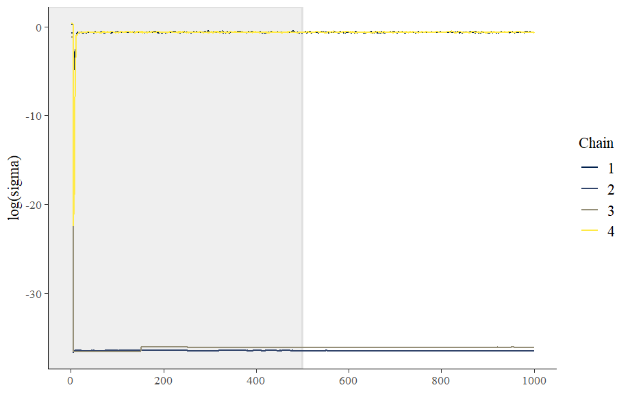
Running the models with non-random inits shows that the affine transform reliably fails when sigma is initialized to low values. The manual version also struggled (with one chain giving me treedepth warnings) but all of the chains converged.

First a check that the models are initializing to the same values as suggested earlier in this thread:

init_test_affine = binom_hier_fit_affine$draws(variables = c("mu", "sigma", "logit_p[1]", "lp__"),  inc_warmup = T)
init_test_raw = binom_hier_fit_raw$draws(variables = c("mu", "sigma", "logit_p[1]", "lp__"), inc_warmup = T)

> init_test_affine[1:6,,"sigma"]
# A draws_array: 6 iterations, 8 chains, and 1 variables
, , variable = sigma

         chain
iteration     1       2        3        4      5    6    7    8
        1 1e-21 4.7e-90 4.4e-159  1.0e-06 0.1210 0.26 0.34 0.80
        2 1e-21 4.7e-90 4.4e-159  1.0e-06 0.1210 0.26 0.34 0.80
        3 1e-21 3.6e-67 4.4e-159  6.7e-04 0.1210 0.26 0.34 0.80
        4 1e-21 1.3e-63 4.7e-159 2.3e-264 0.1210 0.26 0.34 0.80
        5 1e-21 1.3e-63 6.6e-159 2.2e-264 0.0026 0.38 0.45 0.74
> init_test_raw[1:5,,"sigma"]
# A draws_array: 5 iterations, 8 chains, and 1 variables
, , variable = sigma

         chain
iteration       1        2        3        4      5    6    7    8
        1 1.0e-21  2.8e-13  1.0e-10  1.0e-06 0.1210 0.26 0.34 0.80
        2 1.0e-21  2.8e-13  1.0e-10  1.0e-06 0.1210 0.26 0.34 0.80
        3 1.5e-21  2.8e-13  9.4e-09  6.7e-04 0.1210 0.26 0.34 0.80
        4 1.7e-20 9.5e-242 8.5e-153 2.3e-264 0.1210 0.26 0.34 0.80
        5 2.5e-45 1.2e-241 1.1e-152 3.1e-264 0.0026 0.38 0.45 0.74
> init_test_affine[1:5,,"logit_p[1]"]
# A draws_array: 5 iterations, 8 chains, and 1 variables
, , variable = logit_p[1]

         chain
iteration    1     2    3     4    5    6    7   8
        1 0.71 31233 4097   0.7 0.44 0.64 0.55 1.3
        2 0.71 31233 4097   0.7 0.44 0.64 0.55 1.3
        3 0.71 -9704 4097 330.3 0.44 0.64 0.55 1.3
        4 0.71  3404 3699 225.2 0.44 0.64 0.55 1.3
        5 0.71  3404 3524 -18.9 0.64 0.97 1.04 1.7
> init_test_raw[1:5,,"logit_p[1]"]
# A draws_array: 5 iterations, 8 chains, and 1 variables
, , variable = logit_p[1]

         chain
iteration     1    2     3     4    5    6    7   8
        1   0.7 -322   0.7   0.7 0.44 0.64 0.55 1.3
        2   0.7 -322   0.7   0.7 0.44 0.64 0.55 1.3
        3  -3.7 -322 325.2 330.3 0.44 0.64 0.55 1.3
        4 176.4 -133 125.5 225.2 0.44 0.64 0.55 1.3
        5 492.3  209 -56.6  43.0 0.64 0.97 1.04 1.7

That’s a qualified yes, though I’m not sure what’s going on with chains 2 and 3.

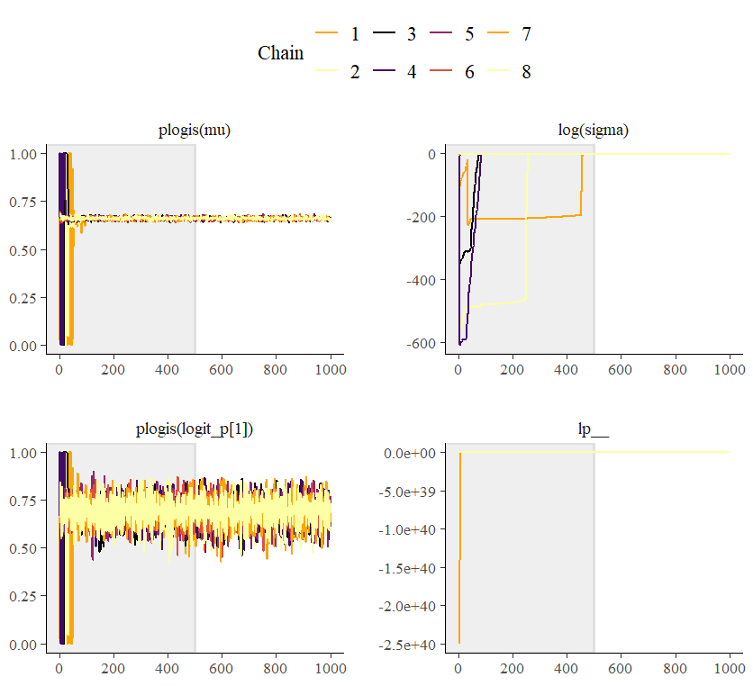
Traceplots. For the affine transform model, all four chains with sigma initialized < 1e-5 got stuck with sigma near-zero, but oddly they all bottomed out far below the initialized values before somewhat recovering.

Here are the traces for manual non-centering model:

Now for something very odd with the the random inits. I was able to pretty quickly hit upon a combination that resulted in a single chain getting stuck at zero for sigma using the affine transform version:

But the initial value for chain 4 was pretty high for sigma. The value provided was 2.26, which got turned into 0.84 for the first few warm-up iterations:

> unlist(c(inits[[1]][2], inits[[2]][2], inits[[3]][2], inits[[4]][2],
+          inits[[5]][2], inits[[6]][2], inits[[7]][2], inits[[8]][2]))
    sigma     sigma     sigma     sigma     sigma     sigma     sigma     sigma 
0.2335458 6.3053346 4.5656075 2.2926901 0.2683244 0.4980496 0.2839859 4.6789906 
> init_test_affine[1:5,,"sigma"]
# A draws_array: 5 iterations, 8 chains, and 1 variables
, , variable = sigma
         chain
iteration       1    2     3    4       5    6       7       8
        1 2.3e-01 2.42 0.026 0.84 2.3e-13 0.43 0.14313 2.8e-01
        2 2.3e-01 2.42 0.026 0.84 2.3e-13 0.43 0.14313 2.8e-01
        3 2.3e-01 2.42 0.026 0.84 2.3e-13 0.43 0.14313 2.8e-01
        4 2.3e-01 2.42 0.026 0.84 2.3e-13 0.43 0.14313 2.8e-01
        5 8.0e-08 0.38 0.148 0.39 8.8e-02 0.29 0.00021 1.5e-15
> init_test_raw[1:5,,"sigma"]
# A draws_array: 5 iterations, 8 chains, and 1 variables
, , variable = sigma

         chain
iteration       1    2     3    4       5    6       7       8
        1 2.3e-01 2.42 0.026 0.84 2.3e-13 0.43 0.14313 2.8e-01
        2 2.3e-01 2.42 0.026 0.84 2.3e-13 0.43 0.14313 2.8e-01
        3 2.3e-01 2.42 0.026 0.84 2.3e-13 0.43 0.14313 2.8e-01
        4 2.3e-01 2.42 0.026 0.84 2.3e-13 0.43 0.14313 2.8e-01
        5 8.0e-08 0.38 0.148 0.39 8.8e-02 0.29 0.00021 4.0e-15

Plotting the paths of the two models for the first 20 iterations (iteration number labelled) and you can see them track each other pretty well at first. But then chain 4 gets stuck for the affine transform. The other two chains (5 and 8) are displayed because for these chains values also started to get down near zero for sigma but then recovered (none of the other chains ever got quite so low). So I’m really not clear what combination of conditions is resulting in the affine transform performing so poorly with this model.

In summary, there is something different about the affine transformation compared to the manual non-centered transform that results in different behavior. Identical initial values and seeds will diverge and it’s not solely a feature of poor initial conditions in terms of sigma being set to zero. However, what’s going on here is a sort of triple transformation (lower bound for sigma, affine/non-centering for the logit_p’s, and then p for binomial. So maybe something pathological in those combinations of constraints?