Number of points with pareto_k > 0.7 increases when a subset of the data set is used

[mmihaylova]

I am fitting a nonlinear mixed-effects model to longitudinal data.
The response variable I am trying to model is the hydrodynamic radius of a an aggregating lipoprotein. The values for the radius are obtained through dynamic light scattering (DLS).
The reason I am explaining this is because the instrument used to measure this radius has a “limit”, after which the measurements are not guaranteed to be very accurate.
The values of the radius measured vary between 15-5000nm.
The recommendation is to usually use values up to a 1000, or slightly more.
So I decided to try out and fit my model twice - once with the whole dataset (with values up to 5000), let’s call it Model1, and once only with values up to 1500 - Model2.

*Note that Model1 and Model 2 are essentially the same model (same fixed and random effects), but priors adjusted for the values in the dataset.
The entire code for the model is given at the end of this post.

The result I got was interesting.

Model1

Family: gaussian
Links: mu = identity; sigma = identity
Formula: LDL ~ 15 + (alpha - 15)/(1 + exp((gamma - Time)/delta))
alpha ~ 1 + (1 | Cat) + (1 | Sample)
gamma ~ 1 + (1 | Cat) + (1 | Sample)
delta ~ 1
Data: Data (Number of observations: 527)
Samples: 3 chains, each with iter = 3000; warmup = 1000; thin = 1;
total post-warmup samples = 6000

Group-Level Effects:
~Cat (Number of levels: 2)
Estimate Est.Error l-95% CI u-95% CI Eff.Sample Rhat
sd(alpha_Intercept) 16.22 12.26 0.64 45.96 5969 1.00
sd(gamma_Intercept) 0.44 0.18 0.09 0.81 1768 1.00

~Sample (Number of levels: 60)
Estimate Est.Error l-95% CI u-95% CI Eff.Sample Rhat
sd(alpha_Intercept) 23.09 17.31 0.89 65.13 3073 1.00
sd(gamma_Intercept) 0.48 0.04 0.42 0.56 930 1.00

Population-Level Effects:
Estimate Est.Error l-95% CI u-95% CI Eff.Sample Rhat
alpha_Intercept 4229.66 122.64 4006.64 4478.77 3687 1.00
gamma_Intercept 2.88 0.19 2.51 3.22 1702 1.00
delta_Intercept 0.44 0.02 0.41 0.47 3487 1.00

Family Specific Parameters:
Estimate Est.Error l-95% CI u-95% CI Eff.Sample Rhat
sigma 382.00 12.29 358.80 407.40 5401 1.00

As one can see, sigma is quite big, which means there would be a lot of uncertainty for the predicted values.

As to the loo output

Computed from 6000 by 527 log-likelihood matrix

     Estimate   SE

elpd_loo -3943.9 47.1
p_loo 99.6 12.1
looic 7887.9 94.2

Monte Carlo SE of elpd_loo is NA.

Pareto k diagnostic values:
Count Pct. Min. n_eff
(-Inf, 0.5] (good) 483 91.7% 833
(0.5, 0.7] (ok) 32 6.1% 220
(0.7, 1] (bad) 10 1.9% 22
(1, Inf) (very bad) 2 0.4% 4
See help(‘pareto-k-diagnostic’) for details.
Warning message:
Found 12 observations with a pareto_k > 0.7 in model ‘model’. With this many problematic observations, it may be more appropriate to use ‘kfold’ with argument ‘K = 10’ to perform 10-fold cross-validation rather than LOO.

Now, 12 bad observations is already a bit worrying, so I looked at the p_loo as well.
The number of parameters I get with parnames() is 133, which means
p_loo < Number of parameters, which, according to this means that my model is likely to be misspecified.
I also run a pp_check, which seemed to reflect the conclusions drawn from loo().

Then I looked at Model2, which was fit only using a subset of the dataset (with values considered to be more accurately measured by the instrument).
Here are the results I got:
Model2

Family: gaussian
Links: mu = identity; sigma = identity
Formula: LDL ~ 15 + (alpha - 15)/(1 + exp((gamma - Time)/delta))
alpha ~ 1 + (1 | Cat) + (1 | Sample)
gamma ~ 1 + (1 | Cat) + (1 | Sample)
delta ~ 1
Data: ldlData (Number of observations: 398)
Samples: 3 chains, each with iter = 6000; warmup = 1000; thin = 1;
total post-warmup samples = 15000

Group-Level Effects:
~Cat (Number of levels: 2)
Estimate Est.Error l-95% CI u-95% CI Eff.Sample Rhat
sd(alpha_Intercept) 15.78 12.10 0.50 44.66 15151 1.00
sd(gamma_Intercept) 0.31 0.19 0.02 0.72 5022 1.00

~Sample (Number of levels: 60)
Estimate Est.Error l-95% CI u-95% CI Eff.Sample Rhat
sd(alpha_Intercept) 183.34 16.29 152.78 216.58 3607 1.00
sd(gamma_Intercept) 0.44 0.04 0.38 0.52 2315 1.00

Population-Level Effects:
Estimate Est.Error l-95% CI u-95% CI Eff.Sample Rhat
alpha_Intercept 1762.20 61.39 1644.00 1884.46 3464 1.00
gamma_Intercept 2.62 0.15 2.35 2.94 7811 1.00
delta_Intercept 0.23 0.01 0.22 0.24 5141 1.00

Family Specific Parameters:
Estimate Est.Error l-95% CI u-95% CI Eff.Sample Rhat
sigma 39.04 2.29 34.56 43.53 3167 1.00

Note that this model was fit using longer chains, however, when using chains with equal length, I got very similar results.

As to the loo output:

Computed from 15000 by 398 log-likelihood matrix

     Estimate   SE

elpd_loo -2161.9 36.6
p_loo 182.5 23.7
looic 4323.8 73.2

Monte Carlo SE of elpd_loo is NA.

Pareto k diagnostic values:
Count Pct. Min. n_eff
(-Inf, 0.5] (good) 297 74.6% 1116
(0.5, 0.7] (ok) 20 5.0% 301
(0.7, 1] (bad) 55 13.8% 34
(1, Inf) (very bad) 26 6.5% 2
See help(‘pareto-k-diagnostic’) for details.
Warning message:
Found 81 observations with a pareto_k > 0.7 in model ‘model’. With this many problematic observations, it may be more appropriate to use ‘kfold’ with argument ‘K = 10’ to perform 10-fold cross-validation rather than LOO.

As one can see, the number of bad observations is really high.
In addition, the number of parameters I obtained with parnames() is 133,
so I have
Number of par. < p_loo, which according to this means that my model is badly misspecified.
I also run a pp_check, the plot of which is given below:

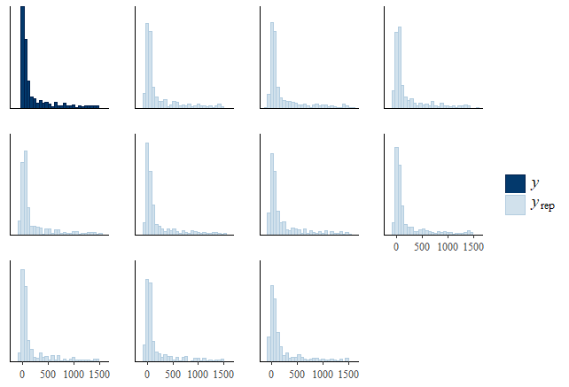
This looks pretty ok to me, much better than the pp_check plots of Model1.
However, in the above link it also said that if p_loo > N/5
(where N is the number of observations) then it is likely for pp_check to not detect the problem, which is probably true in my case.

So I have several questions:

1. Is Model2 badly misspecified?

2. If so, how come Model1, which is essentially the same (with the means and variances of my priors adjusted for the different datasets used), has less pareto_k > 0.7 datapoints?

3. Is it possible for my Model2 to still be useful, but just have higher number of influential observations, due to essentially “cutting out” the higher than 1500 values, essentially leaving the set of data points for each subject looking like this:

which potentially means that potentially the circled point influences the model strongly?

I forgot to mention that the predictions I obtain from Model2 are actually quite reasonable. In addition, I run the model with sample_prior=“only”, and I got no divergences, reasonable Eff. Sample, and Rhats=1.00

The code I’ve used for the model is given below.

fit_model ← function(Data){

fit<- brm(
bf(LDL ~ 15 + (alpha-15) / (1 + exp ((gamma-Time) / delta)),
alpha ~ 1 + (1|Cat) + (1|Sample) ,
gamma ~ 1 + (1|Cat) + (1|Sample),
delta ~ 1,
nl = TRUE),
prior = c(
prior(normal(1500, 30), class=“b”,nlpar = “alpha”),
prior(normal(2.5,0.07), class=“b”, nlpar = “gamma”),
prior(normal(0.2,0.05), class=“b”, lb=0, ub=0.5, nlpar = “delta”),
prior(student_t(3, 0, 10), class=“sigma”),
prior(student_t(3, 0, 10), class=“sd”, nlpar=“alpha”),
prior(student_t(3, 0, 10), class=“sd”, nlpar=“gamma”),
prior(normal(0.4,0.03 ), class=“sd”, group=“Sample”, coef=“Intercept”, nlpar=“gamma”),
prior(normal(300,10), class=“sd”, group=“Sample”, coef=“Intercept”, nlpar=“alpha”),
prior(normal(0.2,0.15), class=“sd”, group=“Cat”, coef=“Intercept”, nlpar=“gamma”),
prior(normal(17,6), class=“sd”, group=“Cat”, coef=“Intercept”, nlpar=“alpha”)),
data = Data, family = gaussian(),
chains = 3,
iter=3000,
warmup = 1000,
cores = getOption(“mc.cores”,1L),
thin = 1,
control = list(adapt_delta = 0.99999, stepsize=0.00001, max_treedepth=15)
)

return(fit)
}

I am not sure if I managed to explain the problem clearly enough, but if anyone is willing to give me some advice, I will happy to answer further questions.

[Max_Mantei]

@mmihaylova

The reason I am explaining this is because the instrument used to measure this radius has a “limit”, after which the measurements are not guaranteed to be very accurate.
The values of the radius measured vary between 15-5000nm.
The recommendation is to usually use values up to a 1000, or slightly more.

Sounds like heteroscedasticity. This would also possibly explains the high values for sigma. (And the much lower values for sigma in your sub-sample.)

Have you tried using, for example, a Gamma distribution with log-link? Or a log-normal? These would only work if you have no zeros in y; If you have zeroes, then a hurdle model would work. I’m pretty sure that these are in brms as well. With both the gamma and log-normal, the variance is assumed to be proportional to the square of the expected (fitted) mean.

Maybe this will also help with the Pareto-k values, as this would naturally put more uncertainty on high measurements.

[mmihaylova]

Hi,

Thank you for your suggestions!
I tried both, but, alas, for some reason I still cannot get good results.
When I tried family=Gamma(link=“log”), I got over 2,000 divergent transitions, so it seems like in this case this is not working.
I also tried family=lognormal(), but this is taking already several hours for 3 chains with 3,000 iterations each, so I am assuming this won’t work, either.

I will play around with the priors some more and see how that goes.

[avehtari]

First it seems you should take into account that LDL is positive. Either with family=lognormal() or making the model for log(LDL) directly.

@mmihaylova

I also tried family=lognormal(), but this is taking already several hours for 3 chains with 3,000 iterations each, so I am assuming this won’t work, either.

If that was the only chance, you could try testing with shorter chains and smalle treedepth whethet you get anything even close to sensible and than just suffer the hours for longer chains.

It’s difficult to estimate how the non-linear function affects the things, but since alpha and gamma both have (1 | Cat) + (1 | Sample), it’s likely that this makes many observations influential especially if the family is badly misspecified. Do you have equal number of observations for each Cat and Sample?

[Max_Mantei]

Did you change the your formula accordingly? With the LogNormal (as well as with the Gamma with log-link) the parameters are on the log scale.

[mmihaylova]

Ah, I didn’t realize that!
Just to double-check, I need to change the priors, as well as take log() of the values of the response variable, correct?

[Max_Mantei]

Yes, to the priors!

No to the taking logs of the response. The inverse link function is applied to the formula, i.e. exp. But your formula already is constrained to be positive as far as I can tell.

However, I don’t see that the equation reduces to something nice and clean when taking logs… but it could well be that I’m missing something here.

EDIT: sorry, had to edit, because I did not read carefully…

Now, that I’m thinking of it… You can also try the Gamma distribution with inverse-link function. Just make sure to apply the inverse-link function to you formula (which in that case would be the inverse).

[mmihaylova]

I am still a bit confused.
So I don’t take logs of the response, but take log of the priors?
And what exactly does the inverse-link do to the model formula?
I am not sure I understand the intuition behind it.

[Max_Mantei]

Take for example a Poisson model. Let say I have Poisson distributed data, Y \sim \text{Poisson}(\lambda), where it has to be that \lambda > 0. For example \lambda = 0.5, or in R:

Y <- rpois(100, 0.5)

Let’s estimate the \lambda using the glm function, we specify link = "identity:

> glm(Y ~ 1, family = poisson(link = "identity"))

Call:  glm(formula = Y ~ 1, family = poisson(link = "identity"))

Coefficients:
(Intercept)  
       0.52 

and get back our estimate for \lambda. For the Poisson GLM link = "log" is actually the default:

> glm(Y ~ 1, family = poisson())

Call:  glm(formula = Y ~ 1, family = poisson())

Coefficients:
(Intercept)  
    -0.6539   

This model is actually estimating \log \lambda = -0.6539 and the inverse link function, i.e. \exp will give us the estimate for \lambda = \exp(-0.6539) = 0.52.

In the first model, if we did it in Stan, we’d to put a prior on \lambda, in the second model, we would have to put a prior on \log \lambda. Note that we didn’t transform the dependent variable.

Now for for a Gamma GLM (the parameters of the Gamma have to be positive, just as in the Poisson case):

> X <- rgamma(100, 1, 1) # implies that estimate should be roughly 1
> glm(X ~ 1, family = Gamma(link = "identity"))

Call:  glm(formula = X ~ 1, family = Gamma(link = "identity"))

Coefficients:
(Intercept)  
       1.27


> glm(X ~ 1, family = Gamma(link = "inverse"))

Call:  glm(formula = X ~ 1, family = Gamma(link = "inverse"))

Coefficients:
(Intercept)  
     0.7871  

In the first model we estimated 1.27. In the second model, we used the inverse transform. As with the log transform above we need the inverse link function to get back the estimate, which in the case of lod was exp. In the case of the “inverse” link, the inverse is the inverse-link (what a sentence). And really, 0.7871^{-1}=1.27. For the Gamma we could also do this:

> glm(X ~ 1, family = Gamma(link = "log"))

Call:  glm(formula = X ~ 1, family = Gamma(link = "log"))

Coefficients:
(Intercept)  
     0.2394  

and apply the inverse-link of the log-link, to get the estimate \exp(0.2394)=1.27.

Often link functions are used if the distribution we want to fit has parameters with restricted range, for example \lambda > 0 of the Poisson. For super simple models like the ones above, link="identity" can work, but usually estimation breaks… Actually, you could try Gamma(link="identity") and maybe it works.

The Log-Normal is kinda special… if you use family = lognormal() you don’t have to transform the dependent variable. If you transform the dependent variable to \log \text{LDL} you can use family = gaussian(link = "identity") (I’d never use a link function with gaussian… this is usually problematic). However, in both cases the formula is like it has a log-link applied to it (as in the Poisson log-link case). Remember in the Poisson log-link case: \exp(\log \lambda)=\exp(-0.6539)=0.52=\lambda: So in a Log-Normal model you are actually estimating \exp(\text{"your model formula"})

So using your model formula in a Log-Normal is estimating \exp( 15 + (\alpha-15) / (1 + \exp ((\gamma-\text{Time}) / \delta)) ), which would be wrong. That means you have to make your formula \log(15 + (\alpha-15) / (1 + \exp ((\gamma-\text{Time}) / \delta)). Now everything is on the log-scale, so you have to think about the parameters/priors in the log-scale.

If you’d use Gamma(link = "inverse") (if that works), then the model is estimating ( 15 + (\alpha-15) / (1 + \exp ((\gamma-\text{Time}) / \delta)) )^{-1} and to “counteract” that you’d have to put your formula through the inverse function (it’s the same, right). It’s late, but if I’m not really stupid, then your model function should then look like this (?): (1 + \exp ((\gamma-\text{Time}) / \delta))/(15 + (\alpha-15))

I really hope I didn’t confuse you even more.

[mmihaylova]

Hi, Max,
Thank you for the thorough explanation (the examples with my model really helped! :))

Now I understand how the lognormal() and the Gamma() family roughly work.
The only thing I am still kind of unsure about is this:

@Max_Mantei

Now everything is on the log-scale, so you have to think about the parameters/priors in the log-scale.

If the lognormal() estimates the exp() of my model and if I deliberately put log(MY MODEL), then I get

exp(log(MY MODEL)) = MY MODEL.

But since the lognormal() has not in any way changed the response values, then it wouldn’t make sense to take logs of the priors I already have, as these would not generate values that are even close to the response values. Or am I mistaken?

[mmihaylova]

I tried with family=lognormal(), bit the results were very strange and quite poor.
The one which gives okay results is family=Gamma(link=“log”).
It only has 10 influential observations, however, even though improved compared to family=lognormal(), are still quite poor.
I played around with the priors, but the results are still not satisfying.

Now, my badly misspecified model actually yields results which are quite OK.
Now, I do realize this is because it is probably wildly overfitted, but in my case that could still be useful. Because one of the things I am actually interested in, is an accurate estimate of gamma (so I assume the overfitted model actually provides a quite good estimate of gamma?).

Now, instead of changing the family and getting a model, whose predictions are quite poor, I was wondering whether I could just do a k-fold with K=10, as the system suggests, and then use the cross-validated model to do predictions?
Would that be a poor way to deal with the problem, or is it actually something I could try out, instead of changing the family and starting from scratch?

[avehtari]

@mmihaylova

Now, instead of changing the family and getting a model, whose predictions are quite poor, I was wondering whether I could just do a k-fold with K=10, as the system suggests, and then use the cross-validated model to do predictions?
Would that be a poor way to deal with the problem, or is it actually something I could try out, instead of changing the family and starting from scratch?

k-fold-cv is a safe choice here for estimating the predictive performance and comparing predictive performances of models. It’s still possible that the model with the best predictive performance has significant mispecification, but at least you don’t need to worry whether Pareto smoothed importance sampling in loo is failing.

[mmihaylova]

I see!
But in this context, what would ‘significant misspecification’ mean, if the model
predicts the values from the dataset quite well, and also gives reasonable predictions for unseen data points, considering the context of the already available data points, does this not make it a reasonably good model?

[avehtari]

I’m intentionally cautious in my words as I can’t confirm it’s a good model without looking at the predictions and data more carefully myself. With k-fold-cv you avoid doubt on PSIS-LOO, but then you still need to know yourself what is “quite well” and “reasonable predictions” in your case.

[Max_Mantei]

You are not the first one to struggle with the Lognormal (I did too for a while). You might want to check out the actually good Wiki article. Note, that the Lognormal has support (0,+\infty), but it’s location parameter has is \mu \in (-\infty,+\infty) – note, that this is not the mean. This is working, because (loosely speaking) the location parameter “runs through” the \exp() function, which maps the input values to the positive real numbers (-\infty,+\infty) \rightarrow (0,+\infty). This means, that \mu is on the log-scale. And that it is called \mu is kinda unfortunate. Well, it does actually make sense, because the way how the log-normal is often defined (in Stan as well) is

\log(Y) \sim \text{Normal}(\mu,\sigma) \leftrightarrow Y \sim \text{LogNormal}(\mu,\sigma).

Well, these are not really equivalent, because in the first you have a change of variables (\log(Y)) and since in Bayesian estimation you are working with probability densities, you need apply the change of variable formula… There is also a tiny section on this in the Stan manual.

Does this make sense?

Also, when I said that you need to take care of the model formula when applying link functions, I was a bit sloppy. I give you two examples from Simon Wood’s fantastic GAM book (Chapter 3, GLMs):

1. Suppose a disease epidemic with relatively few cases (y_i) for now. But the rate of new cases occurring increases exponentially through time. Let \eta_i be the expected number of cases at time t_i, the model is \eta_i = \gamma \exp(\delta t_i). Using a log-link the model becomes \log(\eta_i)=\log(\gamma) + \delta t_i and letting \beta_0 = \log(\gamma) and \beta_1 = \delta, one can write: \log(\eta_i) = \beta_0 + \beta_1 t_i. Note that \beta_0 is now on the log-scale. In R this could look like: glm(y ~ 1 + t, family = poisson(link="log")).

2. The rate of caputre of prey, y_i by a hunting animal increases with density of prey, x_i but levels off eventually when predators catch as much as they are capable of. Let the model by \eta_i=\dfrac{\alpha x_i}{h + x_i}, where \alpha is the max. capture rate and h the prey density at which the max. capture rate is halved. Using a reciprocal (i.e. inverse) link yields 1/\eta_i = \dfrac{1}{\alpha} + \dfrac{h}{\alpha} \dfrac{1}{x_i} = \beta_0 + \beta_1 \dfrac{1}{x_i}, by letting \beta_0=1/\alpha and \beta_1=h/\alpha. In R this could look like this: glm(y ~ 1 + I(1/x), family = Gamma(link="inverse")).

That being said, I’m not sure that this can be neatly done with your model…

[mmihaylova]

Hi,

Thanks again for the extensive answer!
I think this time it is slightly clearer, but I still have some clarifying questions.
For example, I fitted a model and here is its summary:

Family: gamma
Links: mu = inverse; shape = identity
Formula: LDL ~ (1 + exp((gamma - Time)/delta))/(15 + (alpha - 15))
alpha ~ 1 + (1 | Sample)
gamma ~ 1 + (1 | Sample)
delta ~ 1
Data: Data (Number of observations: 368)
Samples: 3 chains, each with iter = 1e+05; warmup = 1000; thin = 1;
total post-warmup samples = 297000

Group-Level Effects:
~Sample (Number of levels: 56)
Estimate Est.Error l-95% CI u-95% CI Eff.Sample Rhat
sd(alpha_Intercept) 299.16 9.98 279.59 318.73 471818 1.00
sd(gamma_Intercept) 0.21 0.03 0.16 0.27 203823 1.00

Population-Level Effects:
Estimate Est.Error l-95% CI u-95% CI Eff.Sample Rhat
alpha_Intercept 1493.99 29.61 1435.94 1551.86 493589 1.00
gamma_Intercept 2.62 0.04 2.55 2.69 282485 1.00
delta_Intercept 0.50 0.00 0.50 0.50 456155 1.00

Family Specific Parameters:
Estimate Est.Error l-95% CI u-95% CI Eff.Sample Rhat
shape 1.68 0.12 1.45 1.92 447832 1.00

Samples were drawn using sampling(NUTS). For each parameter, Eff.Sample
is a crude measure of effective sample size, and Rhat is the potential
scale reduction factor on split chains (at convergence, Rhat = 1).

For this model I have family=Gamma(link=“inverse”).
What confuses me is this line of the output:

Links: mu = inverse; shape = identity

What is mu in this case? Location parameter?

In addition, following your earlier example with the Poisson distribution, since in this case I have link=“inverse”, then for the shape of the Gamma distribution I get
shape = 1/1.68. Or do I keep shape=1.68, as the line above says shape=“identity”?
And, if the latter is correct, do I only take the inverse of mu? And, if so, how do I find mu?

I know I’ve been asking the same question over and over again, but I am still a bit confused about the idea of “family”, as well as the family-related output in summary().