Non-smooth posterior and KKT problem

This is joint work with @shoshievass and follows an earlier discussion: Quadratic optimizier. We’re a little stuck and there are a few open questions. We’ll keep thinking about the issues at hand, but anyone’s welcome to chime in.

As a recap, we want to model optimal bids for an auction. Shosh can fill in the details of the problem or point readers to a reference. As previously discussed, we wrote a quadratic optimizer, which verifies KKT conditions, and exposed it to Stan on a dev branch. See issues 888 on math and 2522 on stan GitHub repos. Using this branch, one can run the quadratic optimizer from cmdStan.

In one of our tests, part of the data generating process involves computing x_p, the solution to a KKT problem. The parameter \gamma controls how many elements of x_p are 0, i.e. at the boundary. In the case where \gamma > 0.5, none of the x_p's are 0, and the unconstrained optimum satisfy the equality and inequality constraints. We simulate data with varying values of \gamma, and fit the same model to the simulated data.

The model fits easily, even as we get (arbitrarily) close to the boundary case, for example when we simulate data with \gamma = 0.6. But, as was suspected notably by @betanalpha, things go south when we hit the boundary, i.e. when we simulate data with \gamma \le 0.5. To be more specific, at \gamma = 0.5:

  • the one x_p that is 0 is correctly estimated as such.
  • the chain does not mix: very little movement in the parameter space, and a high autocorrelation. Increasing the number of sampling iterations from 1000 to 5000 does not help.
  • HMC hits the maximum tree-depth a lot.
  • The chain is slow.
  • There are no divergent transitions.
  • There are no Metropolis proposal rejections.

When \gamma < 0.5 and more than one value of x_p is 0, the sampler only finds one of the inactive values. This suggests the Markov chain gets stuck in a neighborhood of the parameter space.

The above symptoms are all visible in the diagnostic plots, which are attached:
MCMCplot_gamma_06.pdf (26.9 KB)
MCMCplot_gamma_05_1.pdf (21.8 KB)
MCMCplot_gamma_05_2.pdf (21.8 KB)
quadprog_test_5dim.stan (2.8 KB)

And the pairs plot for \gamma = 0.6:

and \gamma = 0.5:

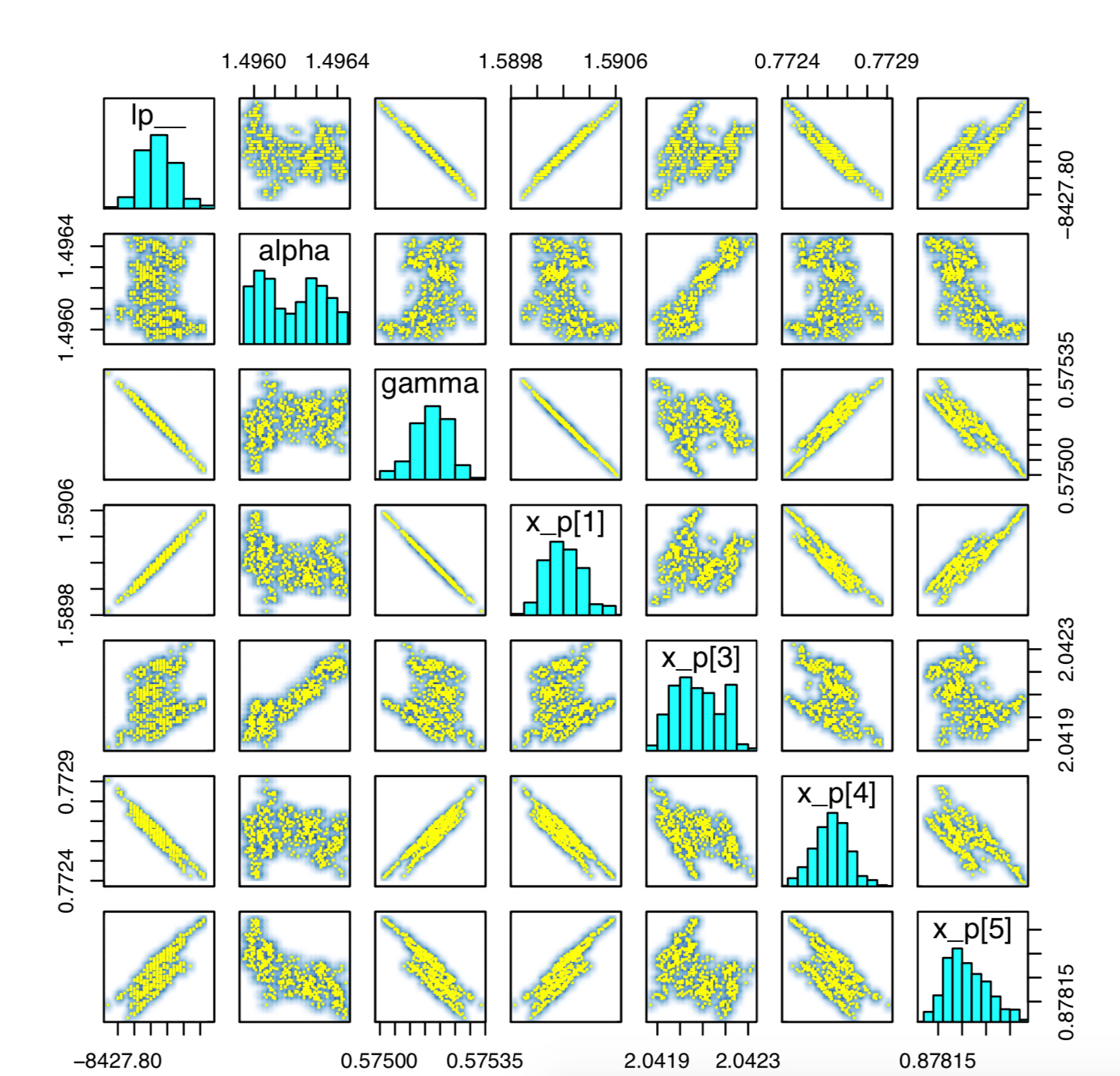
So clearly, the non-smoothness of the joint distribution is hurting us. It is not clear to me exactly why we observe these particular symptoms. I expected the joint to either be roughly smooth, in which case HMC could jump across this boundary; or HMC to spit out divergent transitions, or reject Metropolis proposals because we violate energy conservation when simulating Hamiltonian trajectories.

The next thing I hope to do is work out what the correct posterior would look like. And eventually, think about ways to fit (or approximate) models with this kind of non-smooth structure.

I would suggest one possible solution by combining Zaps to avoid the funnel and model averaging.

A strong boundary-avoid prior adds log-convexity, which is easy to sample from or optimize on. On the other hand, a true zero is also easy to handle. In the end, stacking gives the optimal weights.

Let me explain why this behavior is not unexpected with a simple example.

Consider a one-dimensional problem where the log target density is 0 for x < 0 and 10 for x > 0. Away from zero the Hamiltonian trajectories are given by lines with the kinetic and potential energies constant.

The instant an exact Hamiltonian trajectory passed the boundary at x = 0 the momenta will receive a kick that slows it down or even reverses its direction, manifesting the cost of trying to jump into a region of higher energy. But a numerical Hamiltonian trajectory will jump right past the boundary, miss that kick entirely, and then continue on into the next region unabated. Because the numerical trajectory never sees a large gradient there is no divergence – everything naively looks fine.

But then problems arise when we try to sample from the trajectory. Let’s say that we start in the x < 0 region where the potential energy is zero. All of the points before the boundary have the same Hamiltonian so \Delta H = 0 and we’d sample all of them with the same probability. The points across the boundary, however, have a potential energy of 10 but the same kinetic energy so \Delta H = 10 and the relative sampling probabilities are e^{-\Delta H} = e^{-10}!

In other words the probability that we accept any of the points in the x > 0 region is vanishingly small and we end up sampling points very close to where we started. If we just look at the resulting Markov chain then it looks like it doesn’t go anywhere once it gets close to the boundary.

Things get even worse when adaption is involved. The adaptation algorithm will see the trajectory spending a signifiant time in regions where the acceptance probability is vanishingly small and assume that the integrator is misbehaving because the step size is too big. Consequently it decreases the step size and tries again, but because the vanishingly small acceptance probabilities when transition from x < 0 to x > 0 have nothing to do with the step size the problem doesn’t go away. The adaptation doesn’t know what else to do but lower the step size so it continues stubbornly decreasing it. Ultimately you end up with very small step sizes and corresponding many leapfrog steps for each trajectory.

Putting this altogether one would expect to see

  • No divergences
  • Small step size
  • Treedepth saturation
  • Small transitions away from the initial point
  • Highly autocorrelated Markov chains
    which sounds like a pretty good match to the reputed behavior!

You could try turning adaptation off or decreasing the max_treedepth to limit the size of the trajectories, but then you’d get suboptimal performance away from the boundaries. And even then you’d still be limited by how quickly the momentum resampling could randomly pick a direction that points away from the boundary. Unfortunately, higher-dimensional KKT problems define a polytope where most of the interior looks like a corner where most directions will quickly reach a boundary instead of the desired bulk and these tweaks won’t do much to keep you from getting stuck near the first boundary you encounter.

Ultimately discontinuous target densities are really hiding discrete models with no information about how to efficiently transition from one discrete component to another. Hamiltonian Monte Carlo can’t solve this problem, but its distinct failures do make the problem much easier to identify than with other algorithms. And that’s what really makes it so powerful!

5 Likes

Great, thanks for the insight, this very much agrees with what we observe.

I might add, based on our in-person conversation, that in theory, you could get away with “small” discontinuities. That is, if \Delta H is small enough, you have a decent chance of sampling from your Hamiltonian trajectory passed the discontinuity point. Alternatively, with an asymptotic number of iterations, you’ll eventually sample pass the discontinuity.

None of these considerations seem useful in practice. Any relevant discontinuity incurs a non-negligeable change in the probability density, and therefore a large \Delta H. You could imagine an extreme case where most of the energy is driven by momentum (making \Delta H relatively small), but then you might as well ignore potential all together. And asymptotically does not really help us here if this means running billions of iterations.

The acceptance probability is low because the posterior probability of being past the discontinuity is low! You only want a few samples past the discontinuity, where how few depends on the size of \Delta V. Trying to modify the model to enhance the samples across the boundary fundamentally changes the model and hence its applicability to a given analysis!

The real problem here is that the numerical trajectories miss the opportunity to bounce off of the discontinuity and return back to the bulk, and instead continue forward and waste computation. You end up relying on the momentum resampling to point you in the right direction, and in high-dimensional spaces that can be really inefficient, hence the freezing behavior. Sure, for small enough discontinuities this inefficiency may be small, but in what applications would a tiny discontinuity arise?

The acceptance probability is low because the posterior probability of being past the discontinuity is low!

Yes, I didn’t mean to imply we should change the model to make |\Delta V| go down! It is not clear to me however, that \Delta V is always large – it could also be negative, or small, depending on your model and your data. Of course, if \Delta V is negative you simply get the problem in the other direction.

The real problem here is that the numerical trajectories miss the opportunity to bounce off

We can technically identify a boundary when it is attained: it suffices to check whether a solution attains an unconstrained minimum, or whether it hits one of the constraints. We then monitor this behavior across iterations.

Now, suppose I identify a point or a neighborhood as being close to a boundary. Can I estimate \Delta V, using the probability sampling distribution? I can then treat this as a potential well (or wall rather), and properly simulate Hamiltonian dynamics: if the momentum is large enough I go through, otherwise I bounce back.

There is a lot of overhead in this scheme, but it might be worth trying on the 1d example you described. I can see how this becomes harder in high dimensions, as we might bounce off the boundary multiple times during a single trajectory.

You can identify that you’ve passed a boundary but how do you identify where exactly the boundary is? You can’t root find or apply any other algorithm that would try to iterate between the bounding points to find the boundary because it breaks time reversal invariance.

And then even if you know where the boundary is you’ll need to know it’s geometry – particularly the normal vector to the boundary at any given point – in order to properly bounce. See Section 3.1 of https://arxiv.org/abs/1005.0157 and Appendix A of https://arxiv.org/abs/1112.4118 for more information.