Non-linear mixed effects model specification

[Revathe]

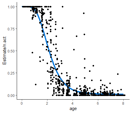
Hi all, I am trying to fit a non-linear mixed effects model to a maternal behaviour. The response variable is a discontinuous proportion. Therefore, it is in the form of a matrix with two columns (resp.mat): 1. no. of successes 2. no. of trials. I want to model this matrix as a function of offspring age and other predictors. The other predictors include offspring sex with two levels, parity with two levels, male status with two levels, and two other continuous predictors. I have one random factor: mother ID. Offspring age has a non-linear effect. Gompertz function fits the non-linear effect well (graph included). I want to add followID as a random factor so that the successes and trials within one follow is treated as a single data point and not multiple data points (which would result in pseudo replication). I have no prior experience with fitting a non-linear mixed effects model. So, I would like some help to understand how to specify the model in brms once I have a function for offspring age, especially with respect to fixed and random effect specification. I am pasting the code I have so far.

gompertz.pred.fun ← function(x, pars){
a = as.vector(pars[“a”])
b = as.vector(pars[“b”])
cc = as.vector(pars[“cc”])
return(1-plogis(a)*exp(-exp(b)*exp(-exp(cc)*x)))
}

gompertz.LL.fun ← function(y, pred.y){
return(-sum(dbinom(x = y[, 1], size=apply(X = y, MARGIN = 1, FUN = sum), prob = pred.y, log = T)))
}

gompertz.both.fun ← function(pars, x, y){
pred.y = gompertz.pred.fun(x = x, pars = pars)
gompertz.LL.fun(y = y, pred.y = pred.y)
}

x = seq(from = 0, to = max(xdata$offspringAge), length.out = 100)
pred.y = gompertz.pred.fun(x = x, pars = c(a = 10, b = 1, cc = 1))
plot(x, pred.y, type = “l”)

gompertz.both.fun(x = xdata$offspringAge, y = xdata$resp.mat, pars = c(a = 10, b = 1, cc = 1))
res = optim(par = c(a = 10, b = 1, cc = 1), fn = gompertz.both.fun, x = xdata$offspringAge, y = xdata$resp.mat)
pred.y = gompertz.pred.fun(x = x, pars = res$par)
plot(x = xdata$offspringAge, y = xdata$resp.mat[, 1]/apply(X = xdata$resp.mat, MARGIN = 1, FUN = sum))
lines(x=x, y=pred.y, col=“red”)

xdata$n.act = apply(X = xdata$resp.mat, MARGIN = 1, FUN = sum)
xdata$n = xdata$resp.mat[, 1]

brm.formula = brmsformula(formula = n|trials(n.act) ~ 1-exp(a)/(1+exp(a))*exp(-exp(b)*exp(-exp(cc)*z.age)), #(1|followID)?
flist = NULL, family = binomial, nl = T, #autocorr=NULL,
a~1+(1|motherID),
b~1+(1|motherID),
cc~1+(1|motherID)
)
get_prior(brm.formula, data = xdata)

priors=c(
set_prior(“normal(4.5, 3)”, class=“b”, nlpar=“a”),
set_prior(“normal(2.5, 3)”, class=“b”, nlpar=“b”),
set_prior(“normal(0.3, 3)”, class=“b”, nlpar=“cc”),
set_prior(“exponential(1)”, class=“sd”, nlpar=“a”, group=“offspringID”),
set_prior(“exponential(1)”, class=“sd”, nlpar=“b”, group=“offspringID”),
set_prior(“exponential(1)”, class=“sd”, nlpar=“cc”, group=“offspringID”),
set_prior(“exponential(1)”, class=“sd”, nlpar=“a”, group=“motherID”),
set_prior(“exponential(1)”, class=“sd”, nlpar=“b”, group=“motherID”),
set_prior(“exponential(1)”, class=“sd”, nlpar=“cc”, group=“motherID”))

Where should priors for followID be included?

Here is the Gompertz function fit to to the data:

[Revathe]

As a follow up, I ran the following model: full.wac=brm(formula=brm.formula, data=xdata, family=“binomial”, prior=priors, control=list(adapt_delta = 0.9))
But I get the following warnings:
Warning messages:
1: Parts of the model have not converged (some Rhats are > 1.05). Be careful when analysing the results! We recommend running more iterations and/or setting stronger priors.
2: There were 170 divergent transitions after warmup. Increasing adapt_delta above 0.9 may help. See Runtime warnings and convergence problems

Could anyone please help with model specification?

[jd_c]

Howdy!
It would help if you provided a reproducible example (the code above can’t be reproduced without xdata.
However, pulling

@Revathe

1-exp(a)/(1+exp(a))*exp(-exp(b)*exp(-exp(cc)*z.age))

from your model formula and using your priors, I can simulate some datapoints implied by those priors for that function:

library(ggplot2)

a <- rnorm(10000, 4.5, 3)
b <- rnorm(10000, 2.5, 3)
cc <- rnorm(10000, 0.3, 3)
z.age <- seq(from=0, to=8, length.out=10000)

y <- 1-exp(a)/(1+exp(a))*exp(-exp(b)*exp(-exp(cc)*z.age))
d <- cbind.data.frame(y, z.age)
ggplot(d, aes(x=z.age, y=y)) + geom_point(size=2)

As can be seen, we obtain y values for different values of z.age from randomly generated values from the prior distributions that you specified in your model. Notice that they imply values that are pretty far from your plot of data and function, which makes me wonder if these values make much sense from your scientific standpoint. For example, is it possible for y to be near zero when z.age is near zero, or for y to be near 1 when z.age is large? That possibility is what your priors imply. This is the concept of prior predictive checks, where you examine the implications of your priors. This is actually easy to do in brms, you simply add in sample_prior="only" to the brm call, run the model sampling from the priors and ignoring the likelihood, and then make plots of model predictions using the pp_check() commands or your own custom plots.

So, I think you should start by doing prior predictive checks, as the priors that you specify for a, b, and cc seem too wide. In addition, the exponential(1) prior that you set for the sd’s is also likely too heavy tailed. You might think about half-normal. Thinking about priors is especially important for non-linear models, as a poor choice may result in the model not converging.

As an example, we could use slightly narrower priors with the same mean as you specified:

a <- rnorm(10000, 4.5, 2)
b <- rnorm(10000, 2.5, 1)
cc <- rnorm(10000, 0.3, 0.15)
z.age <- seq(from=0, to=8, length.out=10000)

y <- 1-exp(a)/(1+exp(a))*exp(-exp(b)*exp(-exp(cc)*z.age))
d <- cbind.data.frame(y, z.age)
ggplot(d, aes(x=z.age, y=y)) + geom_point(size=2)

Does this make more sense from you background knowledge of the subject? The model would likely be identified more easily with these priors than the ones you tried.

[Revathe]

Thank you very much! This makes things so much more understandable now. I am attaching the data that I am using. z.age and predictor 3 are continuous variables. z.age has the non-linear effect. Predictor 2,4,and 5 are categorical with two levels each. Mother ID and follow ID are random factors with 15 and 817 levels, respectively. Could you help me with the model specification? I ran the following model with more informative priors:

brm.formula=brmsformula(formula=n|trials(n.act) ~ (1-exp(a)/(1+exp(a))*exp(-exp(b)*exp(-exp(cc)*z.age))) +
predictor2 + predictor3 + predictor4 + predictor5 ,
flist=NULL, family = binomial, nl=T,#autocorr=NULL,
a~1 + (1|motherID)+ (1|followID),
b~1 + (1|motherID)+ (1|followID),
cc~1 + (1|motherID)+ (1|followID)
)

priors=c(
set_prior(“normal(6.5, 3)”, class=“b”, nlpar=“a”),
set_prior(“normal(3.5, 0.6)”, class=“b”, nlpar=“b”),
set_prior(“normal(0.5, 0.2)”, class=“b”, nlpar=“cc”))

full.wac=brm(formula=brm.formula, data=xdata, family=“binomial”, prior=priors,
control=list(adapt_delta = 0.98))

The fixed effect estimates are not there in the summary, I am not sure why.

Draws: 4 chains, each with iter = 2000; warmup = 1000; thin = 1;
total post-warmup draws = 4000

Group-Level Effects:
~followID (Number of levels: 836)
Estimate Est.Error l-95% CI u-95% CI Rhat Bulk_ESS Tail_ESS
sd(a_Intercept) 0.88 0.66 0.04 2.48 1.00 2423 1995
sd(b_Intercept) 1.71 1.55 0.08 5.55 1.00 3712 2172
sd(cc_Intercept) 0.50 0.37 0.02 1.35 1.00 1803 1456

~motherID (Number of levels: 13)
Estimate Est.Error l-95% CI u-95% CI Rhat Bulk_ESS Tail_ESS
sd(a_Intercept) 1.24 1.10 0.03 4.01 1.00 2125 1496
sd(b_Intercept) 90.97 81.82 25.41 319.38 1.00 2518 1775
sd(cc_Intercept) 1.03 1.01 0.04 3.67 1.00 1961 2027

Population-Level Effects:
Estimate Est.Error l-95% CI u-95% CI Rhat Bulk_ESS Tail_ESS
a_Intercept 12.34 1.67 9.55 16.10 1.00 3566 2418
b_Intercept 3.41 0.60 2.30 4.60 1.00 4602 2697
cc_Intercept 0.47 0.20 0.08 0.86 1.00 5105 2697

Therefore, I am not sure how fixed and random factors should be specified. Are priors necessary for random factors or could I go with the default priors? What would be your suggestion?

The pp_check plot shows that the model performs poorly.

xdata.txt (32.4 KB)

[Revathe]

If it would help, I got the following messages:

Warning messages:
1: In doTryCatch(return(expr), name, parentenv, handler) :
display list redraw incomplete
2: There were 412 divergent transitions after warmup. See
https://mc-stan.org/misc/warnings.html#divergent-transitions-after-warmup
to find out why this is a problem and how to eliminate them.
3: There were 3588 transitions after warmup that exceeded the maximum treedepth. Increase max_treedepth above 10. See
https://mc-stan.org/misc/warnings.html#maximum-treedepth-exceeded
4: Examine the pairs() plot to diagnose sampling problems

[jd_c]

Your data that you have attached looks like a mirror image of you example data, so you will likely need much different priors.

My advice would be to start with the simplest nonlinear model with no random effects, and then after you get it to run well you can try adding the random effects.
You need to do some prior predictive checks and think about how your function works, so that you have a good idea of the priors needed.

[Revathe]

Ah, sorry about that! The original plot was age vs y and not z-transformed age vs y. I have included the original age in the current file. Just a basic question: if my priors are set according to age, can I model with z.age or should I model only with age?

And thank you for your suggestion. I will start with a simpler model.
xdata.txt (42.3 KB)

[jd_c]

If your priors are set according to age, then model with age.
Another problem seems to be the response family. I am not familiar enough with the Gompertz function to make a good suggestion, but I have tried your simple nonlinear model on your data and binomial doesn’t seem to work well.

[Revathe]

Thank you!

I can only think of beta binomial as an alternative since the response is discrete and not continuous. I could try with both binomial and beta binomial.

[jd_c]

I think you need to be using the “identity” link.
Binomial:

m4 <- brm(bf(no_of_successes|trials(no_of_trials) ~ (1-exp(a)/(1+exp(a))*exp(-exp(b)*exp(-exp(cc)*age))),
	a ~ 1, b ~ 1, cc ~ 1, nl=TRUE),
	data=d2, family=binomial("identity"),
	prior=c(
		prior(normal(4.5, 2), class=b, coef="Intercept", nlpar="a"),
		prior(normal(2.5, 1), class=b,  coef="Intercept", nlpar="b"),
		prior(normal(0.3, 0.15), class=b,  coef="Intercept", nlpar="cc")),
	control=list(adapt_delta = 0.95), cores=4)
m4

pp_check(m4, type="hist")

new_data <- cbind.data.frame(age=seq(from=0, to=8, length.out=length(d2$age)), no_of_trials=rep(50, length(d2$age)))
f<-fitted(m4, newdata=new_data)
f<-data.frame(f)
f$age_d2<-d2$age
f$age<-new_data$age
f$no_of_successes <- d2$no_of_successes
f$no_of_trials_d2 <- d2$no_of_trials
f$no_of_trials <- new_data$no_of_trials

p.fit4 <- ggplot(data=f, aes(x=age, y=Estimate/no_of_trials)) + 
	geom_line(size=1.5, color=c("#0275d8")) + 
	geom_ribbon(aes(ymin=Q2.5/no_of_trials, ymax=Q97.5/no_of_trials), fill=c("#0275d8"), size=1.25, linetype="blank", alpha=0.2) +
	theme(panel.grid.major.y = element_blank(), panel.grid.minor.y = element_blank()) +
    	theme(panel.grid.major.x = element_blank(), panel.grid.minor.x = element_blank()) +
    	theme(panel.background = element_rect(fill = "white")) +
    	theme(axis.line.x = element_line(colour = "black")) +
    	theme(axis.line.y = element_line(colour = "black")) +
	geom_point(aes(x=age_d2, y=no_of_successes/no_of_trials_d2), colour="black")
p.fit4

Beta-Binomial:

m6 <- brm(bf(no_of_successes|trials(no_of_trials) ~ (1-exp(a)/(1+exp(a))*exp(-exp(b)*exp(-exp(cc)*age))),
	a ~ 1, b ~ 1, cc ~ 1, nl=TRUE),
	data=d2, family=beta_binomial("identity"),
	prior=c(
		prior(normal(4.5, 2), class=b, coef="Intercept", nlpar="a"),
		prior(normal(2.5, 1), class=b,  coef="Intercept", nlpar="b"),
		prior(normal(0.3, 0.15), class=b,  coef="Intercept", nlpar="cc")),
	control=list(adapt_delta = 0.95), cores=4)
m6

pp_check(m6, type="hist")

new_data <- cbind.data.frame(age=seq(from=0, to=8, length.out=length(d2$age)), no_of_trials=rep(50, length(d2$age)))
f<-fitted(m6, newdata=new_data)
f<-data.frame(f)
f$age_d2<-d2$age
f$age<-new_data$age
f$no_of_successes <- d2$no_of_successes
f$no_of_trials_d2 <- d2$no_of_trials
f$no_of_trials <- new_data$no_of_trials

p.fit6 <- ggplot(data=f, aes(x=age, y=Estimate/no_of_trials)) + 
	geom_line(size=1.5, color=c("#0275d8")) + 
	geom_ribbon(aes(ymin=Q2.5/no_of_trials, ymax=Q97.5/no_of_trials), fill=c("#0275d8"), size=1.25, linetype="blank", alpha=0.2) +
	theme(panel.grid.major.y = element_blank(), panel.grid.minor.y = element_blank()) +
    	theme(panel.grid.major.x = element_blank(), panel.grid.minor.x = element_blank()) +
    	theme(panel.background = element_rect(fill = "white")) +
    	theme(axis.line.x = element_line(colour = "black")) +
    	theme(axis.line.y = element_line(colour = "black")) +
	geom_point(aes(x=age_d2, y=no_of_successes/no_of_trials_d2), colour="black")
p.fit6

Not super great, but a start. I would reiterate the need for good priors on a model like this. Notice that the model still misses the mark for zero successes. You could check this better using something like:

#proportion of zeroes 
prop_zero <- function(x) mean(x == 0)
(prop_zero_testpo <- pp_check(model, type = "stat", stat = "prop_zero"))

[Revathe]

This is a tremendous help! Thank you so much! The identity link makes a lot of sense. I tweaked the priors, and I feel that I have a better fit now.

[Revathe]

This is the model I have now, which runs without any warning messages and the fit seems reasonable (graphs).

brm.formula = brmsformula (formula = n|trials(n.act) ~ 1-exp(a)/(1+exp(a))*exp(-exp(b)*exp(-exp(cc)*age)),
a ~ 1 + (1|motherID),
b ~ 1 + (1|motherID),
cc ~ 1 + (1|motherID),
flist = NULL, nl = T, family = binomial(“identity”)
)

priors = c(
set_prior(“normal(6.5, 1.5)”, class=“b”, coef=“Intercept”, nlpar=“a”),
set_prior(“normal(3.5, 0.6)”, class=“b”, coef=“Intercept”, nlpar=“b”),
set_prior(“normal(0.5, 0.2)”, class=“b”, coef=“Intercept”, nlpar=“cc”),
set_prior(“normal(0,0.2)”, class=“sd”, nlpar=“a”, group=“motherID”),
set_prior(“normal(0,0.2)”, class=“sd”, nlpar=“b”, group=“motherID”),
set_prior(“normal(0,0.2)”, class=“sd”, nlpar=“cc”, group=“motherID”))

m9 ← brm(formula = brm.formula,
data = xdata,
family = binomial(“identity”),
prior = priors,
control = list(adapt_delta = 0.95), cores = 4,
chains = 4, iter = 5000, warmup = 1000)

I want to add the following predictors (xdata.txt): predictor 3 (continuous variables), predictor 2,4,and 5 (categorical with two levels each). Follow ID as a grouping factor with 817 levels. Could someone help me with the model specification and how I could go about setting the priors for these predictors and grouping factor? @paul.buerkner

xdata.txt (42.3 KB)

[jd_c]

@Revathe

I want to add the following predictors (xdata.txt): predictor 3 (continuous variables), predictor 2,4,and 5 (categorical with two levels each). Follow ID as a grouping factor with 817 levels. Could someone help me with the model specification and how I could go about setting the priors for these predictors and grouping factor?

There are different ways to do it. It just depends on how you want your model specified. You could add them to the non-linear formula, but I suspect that you want to add them to the a, b, and/or cc parameters in your Gompertz function. In that case, you would put them in the linear formula for those three parameters in the same way that you did for (1|motherID). Like:

brm.formula = brmsformula (formula = n|trials(n.act) ~ 1-exp(a)/(1+exp(a))*exp(-exp(b)*exp(-exp(cc)*age)),
a ~ 1 + predictor3 + predictor4 + predictor5 + (1|FollowID) + (1|motherID),
b ~ 1 + predictor3 + predictor4 + predictor5 + (1|FollowID) + (1|motherID),
cc ~ 1 + predictor3 + predictor4 + predictor5 + (1|FollowID) + (1|motherID),
flist = NULL, nl = T, family = binomial(“identity”)
)

Of course, you don’t have to include every predictor for every parameter in your non-linear formula. Only include it when it makes sense. Think of the parameters in your non-linear formula as place holders for linear predictors. Then the interpretation for the estimates of those linear predictors is the effect of them on the parameter in the non-linear model.
As for setting priors, you would set them in the same way as you did before. You can use the get_prior() function if you need help figuring out what needs priors. Use domain expertise and prior predictive checks to help decide on priors, as I mentioned in the responses above.

[Revathe]

Thanks a lot!

[Revathe]

I am back again with a few more questions. It will be really helpful to get some guidance. My models have been performing well till I added the random factor (1|followID). Here is the current model and the warning messages.

brm.formula=brmsformula(formula=n|trials(n.act) ~ 1-exp(a)/(1+exp(a))*exp(-exp(b)*exp(-exp(cc)*age)),
a ~ 1 + (1|motherID) + (1|followID),
b ~ 1 + (1|motherID),
cc ~ 1 + predictor2 + predictor4 + predictor5 + predictor3 + (1|motherID),
flist=NULL, nl=T, family=binomial(“identity”)
)

get_prior(brm.formula, data=xdata)

priors=c(
set_prior(“normal(6.5, 1.5)”, class=“b”, coef=“Intercept”, nlpar=“a”),
set_prior(“normal(3.5, 0.6)”, class=“b”, coef=“Intercept”, nlpar=“b”),
set_prior(“normal(0.5, 0.2)”, class=“b”, coef=“Intercept”, nlpar=“cc”),
set_prior(“normal(0,0.2)”, class=“sd”, nlpar=“a”, group=“motherID”),
set_prior(“normal(0,0.2)”, class=“sd”, nlpar=“b”, group=“motherID”),
set_prior(“normal(0,0.2)”, class=“sd”, nlpar=“cc”, group=“motherID”),
set_prior(“normal(0.2,0.4)”, class=“sd”, nlpar=“a”, group=“followID”),
set_prior(“normal(10,1)”, class=“b”, coef=“predictor3”, nlpar=“cc”),
set_prior(“normal(0,1)”, class=“b”, coef=“predictor2M”, nlpar=“cc”),
set_prior(“normal(0,1)”, class=“b”, coef=“predictor4P”, nlpar=“cc”),
set_prior(“normal(0,1)”, class=“b”, coef=“predictor5P”, nlpar=“cc”))

m19 ← brm(formula=brm.formula,
data=xdata,
family=binomial(“identity”),
prior=priors,
control=list(adapt_delta = 0.95, max_treedepth = 15), cores=4,
chains=4, iter=6000, warmup=1000) #increasing the number of iterations

Warning messages:
1: The largest R-hat is 1.66, indicating chains have not mixed.
Running the chains for more iterations may help. See
https://mc-stan.org/misc/warnings.html#r-hat
2: Bulk Effective Samples Size (ESS) is too low, indicating posterior means and medians may be unreliable.
Running the chains for more iterations may help. See
https://mc-stan.org/misc/warnings.html#bulk-ess
3: Tail Effective Samples Size (ESS) is too low, indicating posterior variances and tail quantiles may be unreliable.
Running the chains for more iterations may help. See
https://mc-stan.org/misc/warnings.html#tail-ess

1. Could someone please help with specifying priors for followID?
2. If I want to plot age vs successes/trials and the fitted model, how can I do that for the above model with all the predictors? The conditional_effects plot doesn’t give successes/trials.
3. Finally, if I want to test the significance of this model and get the p value equivalent for each for the predictors, what should I do?

Sorry, I am new to fitting Bayesian models and have little clue about model fitting and inference.

[jd_c]

@Revathe

My models have been performing well till I added the random factor (1|followID).

This is because your data has 850 obs and 817 unique levels of followID. In other words, when you include (1|followID) in your model, you are including a varying intercept for almost every row of data, which makes the model exceedingly flexible and poses great challenges to fit.

@Revathe

Could someone please help with specifying priors for followID?

I would instead consider whether you actually need/desire followID in the model at all. If you do choose to include it, you will need a rather narrow prior for the sd that provides some containment for the weakly informed likelihood. Why do you wish to include followID as a varying intercept?

@Revathe

If I want to plot age vs successes/trials and the fitted model, how can I do that for the above model with all the predictors? The conditional_effects plot doesn’t give successes/trials.

It appears that conditional_effects() is giving the proportion of successes/trials in the plot that you post above…? I am not sure I understand what you are asking… See my code in a previous post above if you wish to make your own plots. You can hold predictors at certain levels or whatever is needed by making your own fake data and then using fitted() or predict() to make predictions (depending on what exactly you want to plot) and them plotting them yourself.

@Revathe

Finally, if I want to test the significance of this model and get the p value equivalent for each for the predictors, what should I do?

Since these are Bayesian models, there aren’t any ‘significance tests’ or p-values. The summary(model) command in brms shows the estimated mean and 2.5% and 97.5% quantiles of the samples from the posterior probability distribution for each parameter. You can also extract the samples using as_draws_df(model) into a dataframe and work directly with them to produce histograms of samples from the posterior distribution or other plots. You can also display your results graphically (like using the conditional_effects() or your own plots).

However, why do you wish to have a significance test or p-value equivalent? What information are you expecting those to provide you that you wish to obtain in this analysis? There are many common misinterpretations of p-values and confidence intervals, and they don’t often provide the information that the researcher thinks they are getting. See Statistical tests, P values, confidence intervals, and power: a guide to misinterpretations - PMC for some good examples.
What you have obtained in your Bayesian model is samples from the posterior probability distributions of the parameters in your model, conditional on the data and model (including priors) that you have specified. This should provide some information about your research question along with some level of statistical uncertainty.

@Revathe

Sorry, I am new to fitting Bayesian models and have little clue about model fitting and inference.

No need to apologize! All good questions. There are a lot of very helpful resources available, including the BDA 3 book, the Statistical Rethinking book (and free YouTube lectures, just search for “Richard McElreath Statistical Rethinking”), and Michael Betancourt’s writing Writing - betanalpha.github.io , just to name a very few.