I’m a bit rusty with my Bayesian analysis, but my understanding is that you need a prior on all parameters. I ran a single-level bernoulli regression with a complementary log-log link function, a discrete-time survival analysis, with the following syntax
brm(formula = event ~ D1 + D2 + D3 + D4 + D5 + D6 + D7 + D8 + D9 + D10 + D11 + gender + group + isi_tot + sf_pain + cpq_tot + qcq_tot + dass_tot + grams_per_day + durationRegUse_dec - 1,
                            family = bernoulli(link = "cloglog"),
                            data = treatDF_PP,
                            seed = 1234)
The analysis worked out great, very similar results to an equivalent NHST analysis. I need to report the priors in the paper, but when I went to examine the stancode using stancode(foo) I got the following
// generated with brms 2.14.4
functions {
  /* compute the cloglog link
   * Args:
   *   p: a scalar in (0, 1)
   * Returns:
   *   a scalar in (-Inf, Inf)
   */
   real cloglog(real p) {
     return log(-log(1 - p));
   }
}
data {
  int<lower=1> N;  // total number of observations
  int Y[N];  // response variable
  int<lower=1> K;  // number of population-level effects
  matrix[N, K] X;  // population-level design matrix
  int prior_only;  // should the likelihood be ignored?
}
transformed data {
}
parameters {
  vector[K] b;  // population-level effects
}
transformed parameters {
}
model {
  // likelihood including all constants
  if (!prior_only) {
    // initialize linear predictor term
    vector[N] mu = X * b;
    for (n in 1:N) {
      // apply the inverse link function
      mu[n] = inv_cloglog(mu[n]);
    }
    target += bernoulli_lpmf(Y | mu);
  }
  // priors including all constants
}
generated quantities {
So where are the priors on mu?
When I read the code under the hood of brms always seems like thrid-dan blackbelt compared to my bluebelt so there’s obviously something going on I don’t understand.
Can someone school me?
In this model, the only parameter (and the only thing that needs a prior) is b (the regression coefficients):
parameters {
  vector[K] b;  // population-level effects
}
When you declare a parameter in Stan and don’t assign a prior in the model block, it is implicitly given a uniform prior across the range of support. So for your model, each element of b is implicitly given a U(-\infty,\infty) prior. If the parameter had been specified with lower and/or upper bounds, the implicit uniform prior is then across those bounds
Thanks @andrjohns, I suspected there might be some default behaviour going on. Much appreciated. Why is it that in brms bernoulli regression has a flat prior by default but standard regression has a weakly-regularising default prior (the t I believe)? And can you suggest a decent weakly-regularising prior for a bernoulli regression with cLoglog link function?
Prior predictive checks really help here. Use the sample_prior = ‘only’ argument in your brms call.
Thank you @franzsf. Can you explain how they help, and what happens when I put that argument into the call?
Basically, you simulate results from your model based only on your priors – i.e. without data. Especially as models get more complicated, priors on individual parameters become harder to interpret. Visual inspection of the prior-only predicted results will tell you how reasonable your prior choices are, given what you know a priori.
If your outcome is heights of human beings, for example, you’d probably want priors that keep most of the predicted results between 0 and 100 ft.
Same thing with bernoulli models - flat priors can push the predicted probabilities to 0 and 1 extremes very quickly. An example of a regularizing prior in the logit space for an intercept-only model would be like a normal(0,2).
Articles like this will do more justice than I could:
https://esajournals.onlinelibrary.wiley.com/doi/full/10.1002/ecs2.3739
Thank you @franzsf, I really appreciate the detail and simplicity, and the reference. So is the idea that you examine the credibility intervals for each coefficient in the prior-only model and if the intervals or point estimates are insane or out of the bounds of theory (e.g. logit coefficients of 200) you revisit your priors?
I read an article by Gelman [http://www.stat.columbia.edu/~gelman/research/published/priors11.pdf] recommending the Cauchy(0,2.5) for logistic regression so I tried that on my model and it also generated sensible results (http://www.stat.columbia.edu/~gelman/research/published/priors11.pdf). How would an intercept-only model affect choice of prior?
I’d say looking at the predicted outcomes with prior predictive simulation is more helpful than looking at individual parameters. Some more resources that might be helpful:
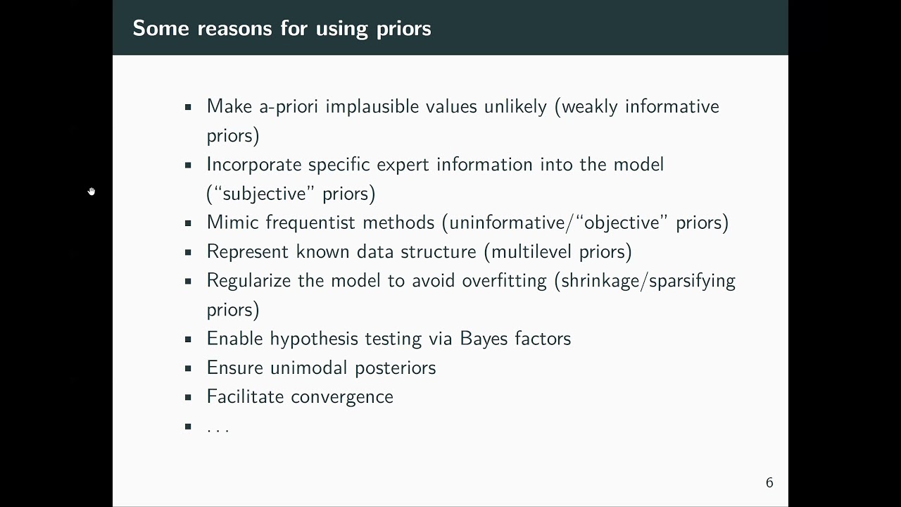
- A talk by Paul Buerkner on priors, which gets into the complexity of setting priors in high dimensional models.
- Also, if you haven’t come across it yet, Richard McElreath’s Statistical Rethinking course (also on Youtube) is one of the best resources out there for introducing folks to Bayesian inference.
