Multi_student_t_rng vs student_t_rng

I am having some trouble with multi_student_t_rng. I might be misunderstanding something simple about multivariate student t distributions, but I assume that if I set the covariance matrix for the multivariate student t distribution to an eye matrix (i.e. ones on the diagonals, zeros elsewhere), then I am effectively generating a collection of K independent student’s t distributions. To check my understanding, I generated some samples using multi_student_t_rng with nu=5, mu=[0, 0]’, and Sigma=[[1,0],[0,1]]. I also generated some samples with student_t_rng with nu=5, mu=0, and sigma=1.

I expected these samples to have the same distribution. However, it looks like they differ. A density plot of the univariate sample matches the pdf of the student’s t distribution, but the multivariate sample does not appear to do so.

I am hoping I have made some trivial mistake, so I can fix it. Code and results follow, and the jupyter lab notebook export is attached. minimal_student_t.html (614.9 KB)

Can anyone spot and explain my mistake, please?

data {
    int nsamp;
    real<lower=0> nu;
}
transformed data {
    matrix[2,2] S = [[1, 0], [0, 1]];
    vector[2] mu = [0, 0]';
}
parameters {}
model {}
generated quantities {
    array[nsamp] vector[2] mult_t;
    array[nsamp] real uni_t;
    mult_t = multi_student_t_rng(nu, rep_array(mu, nsamp), S);
    uni_t = student_t_rng(nu, rep_array(0, nsamp), 1);
}

Here are KDE plots of the two variates in the multivariate sample and of the univariate sample, with the student t pdf from scipy.stats.

image

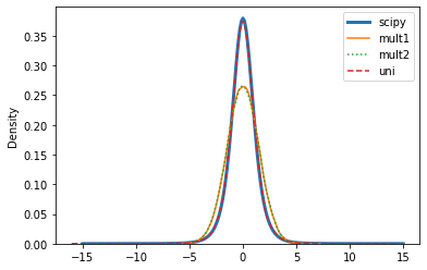
If the colors are hard to see, scipy and uni are on top of each other, and mult1 and mult2 are on top of each other.

1 Like

I don’t know where the error is exactly, but I would suspect the array/matrix broadcasting in multi_student_t_rng(nu, rep_array(mu, nsamp), S)S is 2\times2, but mu is N\times2 and I don’t know why multi_student_t accepts that?

Just to sanity check, I ran the following (which shows the marginals are indeed univariate t):

library(mvtnorm)
library(rstan)
#> Loading required package: StanHeaders
#> rstan (Version 2.26.0.9000, GitRev: 2e1f913d3ca3)
#> For execution on a local, multicore CPU with excess RAM we recommend calling
#> options(mc.cores = parallel::detectCores()).
#> To avoid recompilation of unchanged Stan programs, we recommend calling
#> rstan_options(auto_write = TRUE)
#> For within-chain threading using `reduce_sum()` or `map_rect()` Stan functions,
#> change `threads_per_chain` option:
#> rstan_options(threads_per_chain = 1)
library(magrittr)
#> 
#> Attaching package: 'magrittr'
#> The following object is masked from 'package:rstan':
#> 
#>     extract
library(tibble)
library(ggplot2)

res <- stan(
  model_code = "
  data {
  
  } 
  transformed data {
    matrix[2,2] S = [[1, 0], [0, 1]];
    vector[2] mu = [0, 0]';
  }
  parameters {
  
  } model {
  
  } generated quantities {
  vector [2] mult_t = multi_student_t_rng(3, mu, S);
  real uni_t = student_t_rng(3, 0, 1);
  }
  ",
  chains = 1,
  iter = 1e5 + 1,
  warmup = 1,
  algorithm = 'Fixed_param'
)
#> SAMPLING FOR MODEL 'anon_model' NOW (CHAIN 1).
#> Chain 1: Iteration:      1 / 100001 [  0%]  (Sampling)
#> Chain 1: Iteration:  10000 / 100001 [  9%]  (Sampling)
#> Chain 1: Iteration:  20000 / 100001 [ 19%]  (Sampling)
#> Chain 1: Iteration:  30000 / 100001 [ 29%]  (Sampling)
#> Chain 1: Iteration:  40000 / 100001 [ 39%]  (Sampling)
#> Chain 1: Iteration:  50000 / 100001 [ 49%]  (Sampling)
#> Chain 1: Iteration:  60000 / 100001 [ 59%]  (Sampling)
#> Chain 1: Iteration:  70000 / 100001 [ 69%]  (Sampling)
#> Chain 1: Iteration:  80000 / 100001 [ 79%]  (Sampling)
#> Chain 1: Iteration:  90000 / 100001 [ 89%]  (Sampling)
#> Chain 1: Iteration: 100000 / 100001 [ 99%]  (Sampling)
#> Chain 1: Iteration: 100001 / 100001 [100%]  (Sampling)
#> Chain 1: 
#> Chain 1:  Elapsed Time: 0 seconds (Warm-up)
#> Chain 1:                0.209 seconds (Sampling)
#> Chain 1:                0.209 seconds (Total)
#> Chain 1:

n_plot = 1e4

samples <- rmvt(
  n = 10000,
  df = 3,
  sigma = diag(2)
) %>%
  as_tibble()
#> Warning: The `x` argument of `as_tibble.matrix()` must have unique column names if `.name_repair` is omitted as of tibble 2.0.0.
#> Using compatibility `.name_repair`.

all_samples <- tibble(
  x = c(
    samples$V1[1 : n_plot],
    res %>% rstan::extract(pars = 'mult_t') %>% 
      magrittr::extract2(1) %>%
      magrittr::extract(1 : n_plot, 1),
    res %>% rstan::extract(pars = 'uni_t') %>% 
      magrittr::extract2(1) %>%
      magrittr::extract(1 : n_plot)
  ),
  origin = rep(
    c('mvtnorm', 'multi_student_t_rng', 'student_t_rng'),
    each = n_plot
  )
)

ggplot(data = all_samples) +
  geom_density(aes(x = x, fill = origin), alpha = 0.5) +
  scale_x_continuous(limits = c(-10, 10)) +
  stat_function(
    fun = dt,
    args = list(df = 3)
  )
#> Warning: Removed 65 rows containing non-finite values (stat_density).

Created on 2021-08-04 by the reprex package (v1.0.0)

1 Like

Yeah, it looks like when I do the same thing, I get the same results. That’s encouraging!

I was using this signature:

vectors multi_student_t_rng (real nu, vectors mu, matrix Sigma)
Generate an array of multivariate Student-t variates with degrees of freedom nu, locations mu, and scale matrix Sigma; may only be used in transformed data and generated quantities blocks

from the multivariate student t docs

I thought this was a way to generate many samples with one call, by passing in an array[N] vector[2] I would get an array[N] vector[2] of samples. Edit: Of course, I can accomplish this with a loop, too. I’d still like to know what’s happening with the vectors mu call in the original model, but for now I have a few work-arounds that are just fine.