Model fails to represent uncertainty of test sensitvity/specificity: how to deal with data of different sizes in the likellihood?

The aim of my model is to estimate the prevalence (e.g. of SARS-CoV-2 infection) over time from testing data, adjusting for test sensitivity and specificity. This is indeed a simplified version of my real model, but it is still able to reflect the issue I’m facing.

Let n_i the number of tests performed at week N (i = 1,\dots,N) and y_i the number of tests that are positive. A simple estimated of the prevalence would be y_i/n_i but this does not adjust for imperfect test sensitivity and specificity. We thus followed the method shown by Gelman et al., which takes into account the uncertainy about SARS-CoV-2 PCR test specificity and specificity by simultaneously fitting some specificity/sensitvity data together with the rest of the data.

Using R (version 4.1.3) and CmdStan (version 2.29), I simulated different datasets of number of total and positive tests (n and y) and applied Gelman’s method to estimate the true prevalence. The specificity data consists of 13 studies with an average specificity of 99.5% and the sensitivity data consists of 3 studies showing an average sensitivity of 82.8%.

As a first try, I varied n at around 200. I fixed N=50, with a prevalence varying over time as shown by the dots in the figure below. The model estimates well the observed prevalence (in red), with expected credibility intervals.

mod_example_n200

We also observe that the estimates of the sensitivity and specificity are not modified by the inference, which is what we expect and want, as the test results here (n and y) do not bring any new information on test specificity or sensitivity.

  variable  mean median      sd     mad    q5   q95  rhat ess_bulk ess_tail
  <chr>    <dbl>  <dbl>   <dbl>   <dbl> <dbl> <dbl> <dbl>    <dbl>    <dbl>
1 sens     0.810  0.812 0.0327  0.0331  0.753 0.861  1.00     912.    1395.
2 spec     0.995  0.995 0.00136 0.00134 0.992 0.997  1.00    5054.    2303.

Stan model

data {
  //data to fit
  int N;
  array[N] int n; //number of pools
  array[N] int y; //number of positive pools
  
  //hyperparameters of the priors
  array[2] real p_prev;
  array[2] real p_sens;
  array[2] real p_spec;
  
  //data sensitivity specificity
  int<lower = 0> J_spec;
  array[J_spec] int <lower = 0> y_spec;
  array[J_spec] int <lower = 0> n_spec;
  int<lower = 0> J_sens;
  array[J_sens] int <lower = 0> y_sens;
  array[J_sens] int <lower = 0> n_sens;

  int inference;
} 

parameters {
  //True prevalence
  array[N] real <lower=0,upper=1> prev;
  
  real <lower=0,upper=1> sens; //sensitivity
  real <lower=0,upper=1> spec; //specificity
} 

transformed parameters { 
  //Observed prevalence
  array[N] real <lower=0,upper=1> obs_prev;
  
  for(i in 1:N){
    obs_prev[i] = prev[i] * sens + (1.0-prev[i]) * (1.0-spec);
  }
} 

model {
  //priors
  prev ~ beta(p_prev[1], p_prev[2]);
  sens ~ beta(p_sens[1], p_sens[2]);
  spec ~ beta(p_spec[1], p_spec[2]);
  
  if(inference==1){
    for(i in 1:N){
      target += binomial_lpmf(y[i] | n[i], obs_prev[i]);
    }
  }
  target += binomial_lpmf(y_sens | n_sens, sens);
  target += binomial_lpmf(y_spec | n_spec, spec);
  
}

R script

library(cmdstanr)
library(ggplot)
library(dplyr)
mod = cmdstan_model(stan_file = "mod_example.stan")

#data
time=1:50
prev = 0.1 + 0.6 *time/50 - 0.6*(time/50)^2
plot(time,prev)
n = round(rnorm(50,20000,2000))

stan_data = list(
  N = 50, #number of observations
  n = n, #number of pools
  y = rbinom(50,n,prev), #number of positive pools
  
  p_prev =  c(0.25,1),
  
  J_spec = 13,
  y_spec = c(368,30,70,1102,300,311,500,198,99,29,146,105,50),
  n_spec = c(371,30,70,1102,300,311,500,200,99,31,150,108,52),
  J_sens = 3,
  y_sens = c(78,27,25),
  n_sens = c(85,37,35),
  p_sens = c(1,1),
  p_spec = c(1,1),
  
  inference=0)

# prior
samples_mod =  mod$sample(data = stan_data,
  chains = 4, parallel_chains = 4,adapt_delta=0.99,
  iter_warmup = 1000, iter_sampling = 1000)

#results
samples_mod$summary(c("sens","spec"))

samples_mod$summary(c("prev","obs_prev")) %>% 
  tidyr::separate(variable,"\\[|\\]",into=c("variable","time","null")) %>% 
  mutate(time=as.numeric(time)) %>% 
  dplyr::select(time,variable,median,q5,q95) %>%
  ggplot(aes(x=time)) +
  geom_ribbon(aes(ymin=q5,ymax=q95,fill=variable),alpha=.1) +
  geom_line(aes(y=median,colour=variable),size=1)+
  geom_point(data=data.frame(time=1:50, prev),aes(x=time,y=prev))

# posterior
stan_data$inference=1
samples_mod =  mod$sample(data = stan_data,
                          chains = 4, parallel_chains = 4,adapt_delta=0.99,
                          iter_warmup = 1000, iter_sampling = 1000)

#results
samples_mod$summary(c("sens","spec"))

samples_mod$summary(c("prev","obs_prev")) %>% 
  tidyr::separate(variable,"\\[|\\]",into=c("variable","time","null")) %>% 
  mutate(time=as.numeric(time)) %>% 
  dplyr::select(time,variable,median,q5,q95) %>%
  ggplot(aes(x=time)) +
  geom_ribbon(aes(ymin=q5,ymax=q95,fill=variable),alpha=.1) +
  geom_line(aes(y=median,colour=variable),size=1)+
  geom_point(data=data.frame(time=1:50, prev),aes(x=time,y=prev))

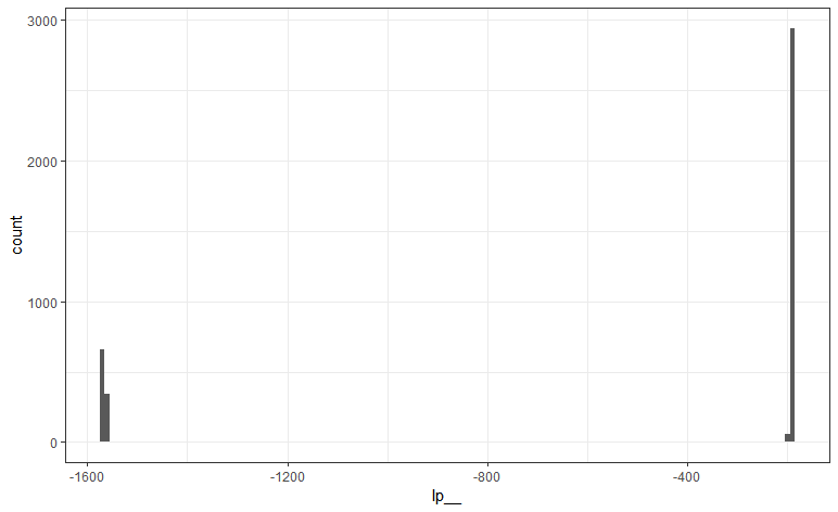
However, when I increase the number of tests n and varied them at around 20,000,

n = round(rnorm(50,20000,2000))

the model gives some weird results, with unexpected estimates of the true prevalence.

mod_example_n20000

When looking at the sensitivity/specificity estimates, we see that the sensitivity is much lower than it should be:

  variable  mean median       sd      mad    q5   q95  rhat ess_bulk ess_tail
  <chr>    <dbl>  <dbl>    <dbl>    <dbl> <dbl> <dbl> <dbl>    <dbl>    <dbl>
1 sens     0.104  0.104 0.00215  0.00211  0.100 0.108  1.00     879.    1557.
2 spec     0.758  0.758 0.000965 0.000961 0.756 0.759  1.00    1207.    2402.

To me, it seems that fitting test data with high n gives too much important to this part of the likelihood and thus, makes the model able to adapt/update the sensitivity estimate. This should not be possible as, as said above, the testing data do not provide any new information about this estimate.

An idea to deal with this kind of issue could be to use a weighted likelihood. I went through this paper, but I’m not sure whether it is quite adapted to my problem and in addition, I do not see how to determine the weights beside the simple binomial example they showed.

Any thought?
Many thanks in advance!
Anthony

1 Like

@andrewgelman @Bob_Carpenter @lucasmoschen

I’d recommend simulating data from the prior and seeing what happens from there. You say that the new data should not be informative about the sensitivity parameter, and I know what you mean, but from a Bayesian perspective the parameters are related.

Taking the extreme of very large N is a good idea in that it should help fix intuition. If you have a large enough N, then you’re estimating Pr(positive test result) exactly, which corresponds to applying a constraint to the prior on the 3-dimensional parameter characterizing sensitivity, specificity, and prevalence. Pr(positive test result) is a nonlinear function of these three parameters, and in general the value you get here will affect your posterior for sensitivity and specificity, as indeed it should, if you think about it that way!

1 Like

Many thanks @andrewgelman for the response!
I am now simulating the data from the priors, except for the prevalence as I wanted it to vary over time (as estimating correctly the sensitivity/specificity only seems to be an issue when the prevalence is not stable over time).

R script

mod = cmdstan_model(stan_file = "R/stan_models/mod_example.stan")

#data
time=1:5
sens = rbeta(length(time), shape1=190,shape2=40)
spec = rbeta(length(time), shape1=1000,1)
prev = 0.01 + 0.3 *time/length(time) - 0.3*(time/length(time))^2
obs_prev = prev * sens + (1.0-prev) * (1.0-spec);
n = round(rnorm(length(time),20000,2000))

stan_data = list(
  N = length(time), #number of observations
  n = structure(n,dim=c(length(n))), #number of pools
  y = structure(rbinom(length(time),n,obs_prev),dim=c(length(n))), #number of positive pools
  
  p_prev =  c(0.25,1),
  
  J_spec = 13,
  y_spec = c(368,30,70,1102,300,311,500,198,99,29,146,105,50),
  n_spec = c(371,30,70,1102,300,311,500,200,99,31,150,108,52),
  J_sens = 3,
  y_sens = c(78,27,25),
  n_sens = c(85,37,35),
  p_sens = c(190,40),
  p_spec = c(1000,1),
  
  inference=0)

# sampling
samples_mod =  mod$sample(data = stan_data,
                          chains = 4, parallel_chains = 4,adapt_delta=0.99,
                          iter_warmup = 1000, iter_sampling = 1000)

samples_mod$summary(c("sens","spec"))


# sampling with inference
stan_data$inference=1
samples_mod =  mod$sample(data = stan_data,
                          chains = 4, parallel_chains = 4,adapt_delta=0.99,
                          iter_warmup = 1000, iter_sampling = 1000)

#results
samples_mod$summary(c("sens","spec","prev"))

Posterior distributions

Even when limiting to 5 time points, the model has issues to estimate the sensitivity:

mod_est <- samples_mod$summary(c("prev","obs_prev")) %>% 
  tidyr::separate(variable,"\\[|\\]",into=c("variable","time","null")) %>% 
  mutate(time=as.numeric(time)) %>% 
  dplyr::select(time,variable,median,q5,q95)

mod_est %>% 
  ggplot(aes(x=time)) +
  geom_ribbon(aes(ymin=q5,ymax=q95,fill=variable),alpha=.1) +
  geom_line(aes(y=median,colour=variable),size=1)+
  geom_point(data=data.frame(time=time, prev),aes(x=time,y=prev)) +
  geom_point(data=data.frame(time=time, obs_prev=obs_prev),aes(x=time,y=obs_prev))

samples_mod$summary(c("sens","spec"))
  variable   mean  median     sd     mad        q5    q95  rhat ess_bulk ess_tail
  <chr>     <dbl>   <dbl>  <dbl>   <dbl>     <dbl>  <dbl> <dbl>    <dbl>    <dbl>
1 sens     0.625  0.817   0.347  0.0321  0.0233    0.855   1.53     7.22     30.7
2 spec     0.981  0.995   0.0252 0.00164 0.937     0.997   1.53     7.21     31.2

Likelihood

I then looked at the distribution of the likelihood and this is surprisingly split into two modes.

samples <- samples_mod$draws() %>%
  as_draws_df() %>%
  as_tibble()

samples %>%
  ggplot(aes(x=`lp__`)) + 
  geom_histogram(binwidth = 10)

samples %>%
  ggplot(aes(x=sens, y=`lp__`)) + 
  geom_point()

To me, two things seem weird:

  1. That the likelihood is separated into two modes (don’t we expect something “continuous” with respect to the parameters?).
  2. That Stan chooses to explore the region with low sensitivity, as the likelihood is very low there. Shouldn’t it focus on the regions with higher likelihood?
    Or am I missing something?
1 Like

What do the various diagnostics (especially R-hat) look like from the run?

Here are the statistics of the main parameters (Rhat is high):

   variable      mean  median      sd     mad        q5    q95  rhat ess_bulk ess_tail
   <chr>        <dbl>   <dbl>   <dbl>   <dbl>     <dbl>  <dbl> <dbl>    <dbl>    <dbl>
 1 sens        0.625  0.817   0.347   0.0321  0.0233    0.855   1.53     7.22     30.7
 2 spec        0.981  0.995   0.0252  0.00164 0.937     0.997   1.53     7.21     31.2
 3 prev[1]     0.111  0.0590  0.0949  0.00396 0.0541    0.311   1.53     7.27     27.9
 4 prev[2]     0.0585 0.0751  0.0316  0.00487 0.0000297 0.0813  1.53     7.23     33.1
 5 prev[3]     0.0616 0.0799  0.0344  0.00503 0.0000184 0.0861  1.53     7.22     35.7
 6 prev[4]     0.142  0.0524  0.159   0.00380 0.0478    0.453   1.53     7.24     36.3
 7 prev[5]     0.254  0.00721 0.429   0.00227 0.00411   1.00    1.53     7.24     30.5
 8 obs_prev[1] 0.0518 0.0518  0.00151 0.00150 0.0493    0.0543  1.01  3197.     2934. 
 9 obs_prev[2] 0.0658 0.0662  0.00265 0.00278 0.0613    0.0697  1.48     7.59     33.0
10 obs_prev[3] 0.0688 0.0702  0.00407 0.00282 0.0614    0.0736  1.53     7.17     29.8
11 obs_prev[4] 0.0464 0.0464  0.00145 0.00145 0.0441    0.0488  1.00  4288.     3302. 
12 obs_prev[5] 0.0132 0.00982 0.00639 0.00105 0.00855   0.0250  1.53     7.16     30.8

And here are the diagnostics:

Checking sampler transitions treedepth.
Treedepth satisfactory for all transitions.

Checking sampler transitions for divergences.
No divergent transitions found.

Checking E-BFMI - sampler transitions HMC potential energy.
The E-BFMI, 0.00, is below the nominal threshold of 0.30 which suggests that HMC may have trouble exploring the target distribution.
If possible, try to reparameterize the model.

The following parameters had fewer than 0.001 effective draws per transition:
  prev[1], prev[2], prev[3], prev[4], prev[5], sens, spec, obs_prev[2], obs_prev[3], obs_prev[5], obs_prev_pred[3], obs_prev_pred[5]
Such low values indicate that the effective sample size estimators may be biased high and actual performance may be substantially lower than quoted.

The following parameters had split R-hat greater than 1.05:
  prev[1], prev[2], prev[3], prev[4], prev[5], sens, spec, obs_prev[2], obs_prev[3], obs_prev[5], obs_prev_pred[2], obs_prev_pred[3], obs_prev_pred[5]
Such high values indicate incomplete mixing and biased estimation.
You should consider regularizating your model with additional prior information or a more effective parameterization.

With such large R-hats and poor ESS, plots like this are more useful for helping to diagnose the problem than to puzzle over as “unexpected”. This looks like a case of some chains getting stuck in the wrong place. Probably a multimodality issue, though this can also happen due to some kinds of numerical issues that cause a chain to get stuck.

1 Like

Ok thanks, point taken. I also noticed that such high Rhat did not occur at every run, which suggests (as you mentionned) that it might be due to numerical issue (right?).
I then reran the model with 50 time points (see my first message), as this one is more likely (it actually always occured at every run) to produce high Rhat and add ‘init=0’, so that the four chains start at the same place. This reduced Rhat for all the parameters. However, some Rhats (for example for the specificity parameter) were still “borderline”, sometimes just higher than 1.05.

So my question is: are there other ways to maximise the chance to have Rhat below 1.05, aside from setting init=0?

R-hat is a very useful diagnostic for difficult posteriors. Making the diagnostic less sensitive doesn’t fix the problem that it’s trying to deal with. That is, your goal is not to force R-hat to be small; it is to deal with the issues in your model that R-hat is helping you to notice.

It seems likely that you are dealing with multimodality here. Default initialization is random, so at random some chains end up in one mode and some chains end up in another. Setting the inits to zero is causing all of the chains to end up in the same mode, but further checking is necessary to better understand

  1. whether the mode they are finding is the “correct” one
  2. whether there even is a “correct” mode with minor modes elsewhere, or whether the is in fact important posterior mass in multiple modes.
  3. how to deal with the resulting computational problem.

If there is a single “correct” mode and other minor modes that are just a computational nuisance, then appropriate initialization might be sufficient to ensure accurate inference. Alternatively, if one of the modes turns out to be inconsistent with your domain knowledge, you could think more carefully about your priors and construct priors that suppress that mode. If there is important posterior mass in multiple modes, all of which are consistent with domain expertise, then your best option for getting accurate inference from this model is to come up with some kind of reparameterization that removes the multimodality, but this isn’t always easy or even possible.