Hello,
I have a mixture model in which I have two distributions (or three if we consider bernoulli and NB_a a mixture itself).
The NB_a has lower center and is zero-inflated, NB_b is distant from 0 and is not zero-inflated.
Having read few posts and the documentation I’m still unsure on how to approach it.
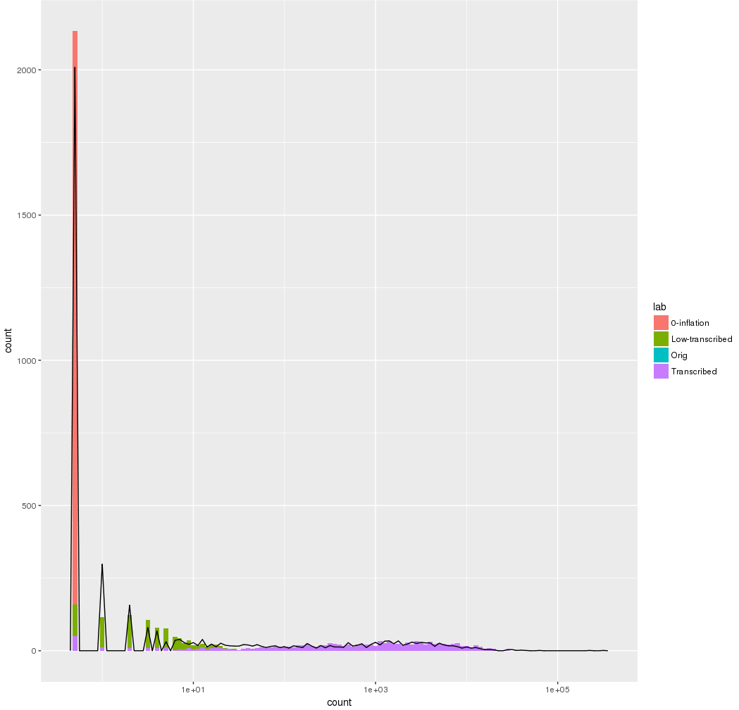
This is LOG plot withOUT zeros
This is LOG plot with zeros (placed as log(0.1)))
Thanks
Does something like this make sense?
  prob_mix =  log_mix(lambda,
	 	neg_binomial_2_lpmf(y[g,s] | mu[1], sigma[1]), //NON
	 	neg_binomial_2_lpmf(y[g,s] | mu[2], sigma[2]) //EXP
	 );

	if (y[n] == 0) target += log_sum_exp(bernoulli_lpmf(1 | theta), bernoulli_lpmf(0 | theta) + prob_mix);
	else target += bernoulli_lpmf(0 | theta)	+ prob_mix;
for (n in 1:N)
   target += log_mix(lambda
    	 	, y[n] == 0 ? log((1-theta) * exp(neg_binomial_2_lpmf(y[n] | mu[1], sigma[1])) + theta)
                               : log1m(theta) + neg_binomial_2_lpmf(y[n] | mu[1], sigma[1])
    	 	, neg_binomial_2_lpmf(y[n] | mu[2], sigma[2])
    	 );
It can be optimized with log_sum_exp.
Andre
Hi Andre –
It seems a bit counter-intuitive to include a zero-inflated negative binomial in a mixture of negative binomials because a zero-inflated model is also a mixture. A negative binomial model can handle situations with spikes and exponential-type tails, so the zero inflation may be overkill in this situation.
But if you do want a separate model for zeroes, then I think a possible solution would be to do something like the following. This code assumes that the location for the negative binomial models can be transferred to the zero-inflated models, which are mixtures of bernoulli (logits):
if(y[n]==0) {
target += log_mix(lambda_zero,bernoulli_logit_lpmf(0 | mu[1]),
                    bernoulli_logit_lpmf(0 | mu[2]));

} else {
target += log_mix(lambda_zero,bernoulli_logit_lpmf(1 | mu[1]),
                    bernoulli_logit_lpmf(1 | mu[2]));
target += log_mix(lambda,insert neg binomial mixture here);
}
You could keep lambda as the same parameter between both sets of mixtures as well.
A mixture of a Dirac mass at zero and two negative binomials is fine provided that the priors ensure that the two negative binomials do not peak at zero. And it would be easier to treat this as a three way mixture with a simplex instead of trying to mix them sequentially, first into a zero-inflated negative binomial and then with another negative binomial as proposed in the question.
Is it really possible write this directly as a three way mixture with a single simplex?
What I mean is, it’s straightforward if it’s just two (or more) NBs without inflation where we would have:
(y_i | H_i = j) ~ NB(mu_j, phi_j)
and the usual hierarchical structure:
P(H_i = j | lambda_j) = lambda_j
lambda ~ Dirihlet(…)
But if we have inflation, I don’t see a way to it directly as a new “cluster” like we would do for an another NB cluster, the only way I see past this would be create a Bernoulli random variable that would “switch” between the inflation and the rest of the mixture (that is, a zero inflated finite mixture model).
Thanks,
yes I though of the 3 way mixture with the 0 inflated treated as another NB, but didn’t work well.
I will try to implement the three options you guys suggested and take care of the means of the two NB to be > 0.
Hello @saudiwin I was just trying to understand:
-
is there any relation between the two mu, and the other center of NB within the mix “insert neg binomial mixture here”
-
basically I will have 4 lambda, I don’t understand how could I treat lambda_zero as lambda, they will be necessarily different (?)
Thanks
This is for sure a dummy question but what it the best prior for bernoulli_logit_lpmf?
thanks
Hello,
I have tried this implementation.
data {
	int<lower=1> G;
  int y[G]; // data. gene mupression (integer counts)
}

parameters {
positive_ordered[2] mu; // prior location
real mu_zero[2];

real<lower=0> sigma[2];
real<lower=0, upper=1> lambda;
real<lower=0, upper=1> lambda_zero;

}
model {

for(g in 1:G){
if(y[g]==0) {
	target += log_mix(lambda_zero,bernoulli_logit_lpmf(0 | mu_zero[1]),
	                    bernoulli_logit_lpmf(0 | mu_zero[2]));

} else {
	target += log_mix(lambda_zero,bernoulli_logit_lpmf(1 | mu_zero[1]),
	                    bernoulli_logit_lpmf(1 | mu_zero[2]));
	target += log_mix(lambda,
		neg_binomial_2_lpmf(y[g] | mu[1], sigma[1]), //NON
	 	neg_binomial_2_lpmf(y[g] | mu[2], sigma[2]) //EXP
	 	);
}
}

		sigma ~ gamma(1.1, 2);
		mu[1] ~ gamma(2, 0.1);
		mu[2] ~ gamma(2, 0.001);
		lambda ~ beta(2,2);
		mu_zero ~ cauchy(0,2);
}
generated quantities{
	int y_hat_1;
	int y_hat_2;

	y_hat_1 = neg_binomial_2_rng(mu[1], sigma[1]);
	y_hat_2 = neg_binomial_2_rng(mu[2], sigma[2]);

}
But although the lambda proportion is plausible, the model have n_eff of 1000. What am I doing wrong?
$summary
                     mean      se_mean           sd          2.5%           25%           50%           75%         97.5%      n_eff
mu[1]        2.013666e+00 3.115304e-05 9.851458e-04  2.011707e+00  2.013001e+00  2.013643e+00  2.014335e+00  2.015687e+00 1000.00000
mu[2]        2.013817e+00 3.108038e-05 9.828478e-04  2.011894e+00  2.013176e+00  2.013792e+00  2.014474e+00  2.015836e+00 1000.00000
mu_zero[1]   4.950094e-01 3.523073e-01 3.287522e+00 -5.046529e+00 -5.889891e-01 -2.383201e-02  9.439835e-01  1.063341e+01   87.07513
mu_zero[2]   4.976698e-01 3.210963e-01 3.631214e+00 -5.006008e+00 -6.284321e-01 -2.724642e-03  8.411252e-01  1.155646e+01  127.88900
sigma[1]     2.231683e-01 1.176291e-04 3.719758e-03  2.157514e-01  2.206539e-01  2.231813e-01  2.256023e-01  2.306998e-01 1000.00000
sigma[2]     3.706016e-04 9.779321e-08 3.092493e-06  3.643050e-04  3.684997e-04  3.707494e-04  3.727237e-04  3.763318e-04 1000.00000
lambda       5.222136e-01 9.710504e-05 3.070731e-03  5.162808e-01  5.201050e-01  5.222999e-01  5.241679e-01  5.284114e-01 1000.00000
lambda_zero  5.042542e-01 2.797127e-02 2.630855e-01  2.747268e-02  3.109872e-01  5.054078e-01  6.916956e-01  9.690703e-01   88.46455
y_hat_1      1.933000e+00 1.307425e-01 4.134441e+00  0.000000e+00  0.000000e+00  0.000000e+00  2.000000e+00  1.500000e+01 1000.00000
y_hat_2      2.088000e+00 2.049091e+00 6.479796e+01  0.000000e+00  0.000000e+00  0.000000e+00  0.000000e+00  0.000000e+00 1000.00000
lp__        -3.559931e+05 3.327286e-01 2.442393e+00 -3.559989e+05 -3.559945e+05 -3.559928e+05 -3.559912e+05 -3.559894e+05   53.88289
                 Rhat
mu[1]       1.0027428
mu[2]       1.0031876
mu_zero[1]  1.0672225
mu_zero[2]  1.0570077
sigma[1]    0.9972462
sigma[2]    0.9980175
lambda      0.9984677
lambda_zero 1.0083174
y_hat_1     0.9967248
y_hat_2     1.0000279
lp__        1.0763487
Can the problem be that I have high count values to start with ?
> summary(mix[,1])
     Min.   1st Qu.    Median      Mean   3rd Qu.      Max.
      0.0      11.5      73.3    1394.0     277.0 2559000.0
Haven’t check the model, but maybe it has to do with your prior for sigma? I would try a half-cauchy as prior for sigma and also Poisson components instead of NBs.
Zero-inflated Poisson might be “general” enough for your case by being capable of capturing overdispersion and therefore ZINB might be a hard to fit “overkill” (and here you even have two components NB), specially with a prior that places strong probability that phi is near zero (far from the Poisson case). I had some nightmares in the past with a overdispersed zero-inflated dataset that also presented low n_eff and actually needed to increase max_treedepth of NUTS (check if your current fitted model exceeded it), but it was zero-inflated regression of car insurance dataset (ridiculous amount of zeros and overdispersion).
Thanks I will try.
What is the best prior for mu_zero (bernoulli_logit) in my case?
Hi Steman –
I don’t know why you’re saying that n_eff is low… remember that n_eff is only counting based on post-warmup iterations, so it depends how many iterations from all chains post-warmup. 1000 is a great number for estimating parameters with high precision.
It looks like the zero-inflation part isn’t mixing super well, but that’s because there’s very little information to fit two models to the 0/1 part of the model. That’s why I suggested keeping the means mu the same between the negative binomial and bernoulli models on the assumption that the same process that will increase the mean of the negative binomial will increase the probability of 1 for the bernoulli distribution.
Any prior centered around 0 with a small sd works fine for logit because logit(0) = 0.5 probability.
Honestly, I don’t see much wrong with your model other than that the R-hat on the log-posterior is 1.07-- you might want to run the sampler another 1,000 iterations to bring that down, but otherwise there are no serious pathologies even if you could work more on the zero-inflation part.
Thanks Saudiwin,
now the model is working fine
except is pretty slow.
This part can be modified
for(g in 1:G){
if(y[g]==0) {
	target += log_mix(lambda_zero,bernoulli_logit_lpmf(0 | mu_zero[1]),
	                    bernoulli_logit_lpmf(0 | mu_zero[2]));

} else {
	target += log_mix(lambda_zero,bernoulli_logit_lpmf(1 | mu_zero[1]),
	                    bernoulli_logit_lpmf(1 | mu_zero[2]));
	target += log_mix(lambda,
		neg_binomial_2_lpmf(y[g] | mu1, si1), //NON
	 	neg_binomial_2_lpmf(y[g] | mu2, si2) //EXP
	 	);
}
}
to
target += log_mix(lambda_zero,bernoulli_logit_lpmf(0 | mu_zero[1]),
	                    bernoulli_logit_lpmf(0 | mu_zero[2])) *     NUMBER_OF_ZEROS;
target += log_mix(lambda_zero,bernoulli_logit_lpmf(1 | mu_zero[1]),
	                    bernoulli_logit_lpmf(1 | mu_zero[2]))* NUMBER_OF_NON_ZEROS;
for(g in 1:NON_ZEROS){
    	target += log_mix(lambda,
    		neg_binomial_2_lpmf(y[g] | mu1, si1), //NON
    	 	neg_binomial_2_lpmf(y[g] | mu2, si2) //EXP
    	 	);
    }
    }
Mixture models aren’t vectorized in Stan, so unfortunately there is no way to speed up the model without simplifying it (i.e., dropping components).
But I though this was not a vectorization.
I am just representing for loops in a compressed way, The sum of lpdf of the log_mix for bernoulli does not change.
From -2 -2 -2 -2 -2 -2 becomes -2 * 6
Then it will no longer be a mixture of Bernoulli’s. See the Stan manual on
mixtures.