Lognormal Hierarchical Distribution Fitting

Hi All, I’m just getting started with Stan and I’m having a little trouble. The thing I’m interested in doing is basically hierarchical distribution fitting of insurance claim amounts by state. I’ve simulated (from a lognormal distribution) 50 claim amounts for the state of IL, 20 in the state of WI, and 5 in the state of MN, with each state having different lognormal parameters mu and sigma. From what I’ve read, the hierarchical approach should get me to a credibility weighting between a pooled (all states combined) and unpooled (each state individually) estimate for each state. So for IL I would expect the parameter estimates to be closer to the unpooled estimates because it has 50 claims and MN should be closer to the pooled estimate because it has only 5 claims.

I’ve included the stan code for 3 different models below. I first run a pooled version, then each state individually, then an unpooled version, and then the partial pooling version. I ran each state individually and then compared that to the unpooled estimates to help me understand if I was creating the unpooled model correctly but also to verify that I got the same parameter estimates. They are pretty close, but don’t match exactly. So that is my first question: why don’t the unpooled estimates for each state match the individual state estimates?

My second question stems from the fact that I don’t observe the hierarchical estimates being between the pooled and unpooled estimates. Is there a problem with my hierarchical model which would cause this exercise I’m trying to go through to fail, or am I misunderstanding this exercise from the start? I realize that it’s ending up with different hyperparameter estimates for my gamma priors than what I’m using in my pooled and unpooled versions so I did re-run it all hard coding in the mean estimates from the hierarchical model into the gamma priors in the pooled and unpooled models but that didn’t have a big impact and didn’t solve the problem.

Like I said, I’m just getting started with stan and appreciate any help here. All code is included below.

First up, the pooled model (also used to do each state individually):

//lognormal_pooled.stan
data {
  int<lower=1> N; //number of records
  real<lower=0> y[N]; //outcomes (loss amounts)
}
parameters {
  real mu;
  real<lower=0> sigma;
}
model {
  //priors
  mu ~ gamma(9, 1);
  sigma ~ gamma(2, 1);
  //likelihood
  y ~ lognormal(mu, sigma);
}
} 

Next, the unpooled model:

//lognormal_unpooled.stan
data {
  int<lower=1> N; //number of records
  int<lower=1> K; //number of groups (states)
  int<lower=1,upper=K> state[N]; //vector of state values
  real<lower=0> y[N]; //outcomes (loss amounts)
}
parameters {
  real mu[K];
  real<lower=0> sigma[K];
}
model {
  //priors
  mu ~ gamma(9, 1);
  sigma ~ gamma(2, 1);
  //likelihood
  for (n in 1:N){
    y[n] ~ lognormal(mu[state[n]], sigma[state[n]]);
  }
}

Lastly, the hierarchical model (or my attempt at it):

//lognormal_partial_pooling.stan
data {
  int<lower=1> N; //number of records
  int<lower=1> K; //number of groups (states)
  int<lower=1,upper=K> state[N]; //vector of state values
  real<lower=0> y[N]; //outcomes (loss amounts)
}
parameters {
  real<lower=0> mu_alpha;
  real<lower=0> mu_beta;
  real<lower=0> sigma_alpha;
  real<lower=0> sigma_beta;
  real mu[K];
  real<lower=0> sigma[K];
}
model {
  //priors  
  mu_alpha ~ gamma(9, 1);
  mu_beta ~ gamma(1, 1);
  sigma_alpha ~ gamma(2, 1);
  sigma_beta ~ gamma(1, 1);
  mu ~ gamma(mu_alpha, mu_beta);
  sigma ~ gamma(sigma_alpha, sigma_beta);
  //likelihood
  for (n in 1:N){
    y[n] ~ lognormal(mu[state[n]], sigma[state[n]]);
  }
}

Below is the R code I’m using:

library(rstan)
library(data.table)
# pkgbuild::has_build_tools(debug = TRUE)
options(mc.cores = parallel::detectCores())
rstan_options(auto_write = TRUE)

set.seed(20200402)
dt <- data.table(rbind(data.frame(state = "IL", loss = rlnorm(50, 10, 3)),
            data.frame(state = "WI", loss = rlnorm(20, 9, 2)),
            data.frame(state = "MN", loss = rlnorm(5, 8, 1.5))))
dt[, state_id := .GRP, by = state]
pooled_data <- list(N = nrow(dt),
                    y = dt[, loss])
pooled_data_IL <- list(N = nrow(dt[state == "IL"]),
                       y = dt[state == "IL", loss])
pooled_data_WI <- list(N = nrow(dt[state == "WI"]),
                       y = dt[state == "WI", loss])
pooled_data_MN <- list(N = nrow(dt[state == "MN"]),
                       y = dt[state == "MN", loss])
unpooled_data <- list(N = nrow(dt),
                      K = dt[, max(state_id)],
                      state = dt[, state_id],
                      y = dt[, loss])

pooled_fit <- stan(file = 'lognormal_pooled.stan', data = pooled_data)
pooled_fit_IL <- stan(file = 'lognormal_pooled.stan', data = pooled_data_IL)
pooled_fit_WI <- stan(file = 'lognormal_pooled.stan', data = pooled_data_WI)
pooled_fit_MN <- stan(file = 'lognormal_pooled.stan', data = pooled_data_MN)
unpooled_fit <- stan(file = 'lognormal_unpooled.stan', data = unpooled_data)
partial_pooling_fit <- stan(file = 'lognormal_partial_pooling.stan', data = unpooled_data)

summary(pooled_fit_IL)$summary[, "mean"]
summary(pooled_fit_WI)$summary[, "mean"]
summary(pooled_fit_MN)$summary[, "mean"]
summary(unpooled_fit)$summary[, "mean"]
summary(pooled_fit)$summary[, "mean"]
summary(partial_pooling_fit)$summary[, "mean"]
3 Likes

Hey! Welcome to the Stan forum!

That’s a well stated first question, thank you! :)

Before diving in, there are 4 things I noticed.

  1. The \mu and \sigma parameters of the lognormal in Stan are on the log scale – just as in the rlnorm R function. Putting gamma priors on the \mu parameter implies that you neglect parts of the possible parameter space. This can be fine, but usually (especially with hierarchical models) you want them to be a bit more flexible.
  2. I think conventional partial pooling models don’t partial pool the \sigma of the outcome (the sigma that goes into the lognormal). Again, it’s not necessarily wrong to do that, but you probably want to start with just partial pooling \mu and leave \sigma as the observational level uncertainty.
  3. Usually, I use normal distribution for the priors, e.g. \mu \sim \text{Normal}(\mu_0, \sigma_\mu), so that \mu_0 is the values everything is pulled towards (especially low-observation groups), and \sigma_\mu gives an indication of overall pooling taking place.
  4. How are model diagnostics? Divergent transitions etc.? Sometimes reparameterization is necessary – which are easier if you use normal distributions as hierarchical priors (see 3.).

Feel free to ask follow ups. I might be able to run the models myself later or tomorrow.

Cheers,
Max

3 Likes

Thanks for the response, Max_Mantei! I’ve responded to your points below.

To caveat this, lognormal is the first distribution that I’m working with on this exercise. My aim will be to create other versions of this for other distributions common to the insurance industry, like Pareto, Gamma, Weibull, etc. Eventually I want to be able to look at mixtures of these models as well. As I get to those,

  1. That’s fair. \mu \in (-\infty,+\infty) so seems like Normal would make sense. I’ve gone through and changed my prior in my pooled and unpooled models to use \mu \sim Normal(9,3).
  2. I did consider this but there can be good reasons why we expect different variability by state, so initially left it just to see how well the \sigma parameters would get recovered. As I get this off the ground that will be a modeling consideration that I’ll explore more. However, I’ve attempted to do this in my partial pooling model below.
  3. This is something I may need a little more background on. How does \sigma give an indication of the pooling taking place? It may be that I haven’t rewritten this correctly based on what you’re recommending. Feel free to set me straight :-)
  4. Admittedly, I’m not very comfortable with assessing model diagnostics in this framework yet. When I first started I get a bunch of warnings about divergent transitions. Now, with the code I provided, I don’t get any warnings like that. However, when I use the get_sampler_params function in RStan I do see there’s a small number of divergent transitions. I’d be happy for you to share a set of standard diagnostics that you look at!

My revised partial pooling model is below. I commented out the old stuff so you can see the changes I made.

//lognormal_partial_pooling.stan
data {
  int<lower=1> N; //number of records
  int<lower=1> K; //number of groups (states)
  int<lower=1,upper=K> state[N]; //vector of state values
  real<lower=0> y[N]; //outcomes (loss amounts)
}
parameters {
  real<lower=0> mu_alpha;
  //real<lower=0> mu_beta;
  //real<lower=0> sigma_alpha;
  //real<lower=0> sigma_beta;
  real mu[K];
  //real<lower=0> sigma[K];
  real<lower=0> sigma;
}
model {
  //priors  
  //mu_alpha ~ gamma(9, 1);
  mu_alpha ~ normal(9, 3);
  //mu_beta ~ gamma(1, 1);
  //sigma_alpha ~ gamma(2, 1);
  //sigma_beta ~ gamma(1, 1);
  //mu ~ gamma(mu_alpha, mu_beta);
  mu ~ normal(mu_alpha, 3);
  //sigma ~ gamma(sigma_alpha, sigma_beta);
  sigma ~ gamma(2, 1);
  //likelihood
  for (n in 1:N){
    //y[n] ~ lognormal(mu[state[n]], sigma[state[n]]);
    y[n] ~ lognormal(mu[state[n]], sigma);
  }
}

After making these changes my original 2 questions still stand. My output is below. If we look at the \mu for IL, for example. I simulated the values in R with \mu=10, the true value. When I estimate just using IL data (pooled_fit_IL), I get an estimate of \mu=10.018528, which is pretty close to the true value. When I run my unpooled model (unpooled_fit), which I believe should be equivalent to running each state through individually, I get \mu=10.038347, which is close but not the same to the individually run estimate. That’s still my first question: why aren’t these equal? Have I not correctly set up my unpooled model, or is there a good reason as to why it wouldn’t be the case?

For my second question, I do see that the estimates for \mu using partial pooling are all between the corresponding unpooled estimates and the pooled estimate. However, MN looks odd to me. There’s only 5 claims for MN out of the 75 total claims for all states, yet the partial pooling estimate is much closer to the unpooled estimate than the pooled estimate: \mu_{unpooled}=7.150575 < \mu_{partial}=7.352847 < \mu_{pooled}=9.674004. I would expect this state to get shrunk towards the all-states-combined estimate due to low volume of observations. This makes me think I haven’t correctly set up my hierarchical model. Any thoughts?

> summary(pooled_fit_IL)$summary[, "mean"]
        mu      sigma       lp__ 
 10.018528   3.243219 -85.167946 
> summary(pooled_fit_WI)$summary[, "mean"]
        mu      sigma       lp__ 
  9.422599   2.026193 -24.494303 
> summary(pooled_fit_MN)$summary[, "mean"]
       mu     sigma      lp__ 
 7.128955  1.572030 -5.238653 
> summary(unpooled_fit)$summary[, "mean"]
      mu[1]       mu[2]       mu[3]    sigma[1]    sigma[2]    sigma[3]        lp__ 
  10.038347    9.427064    7.150575    3.231905    2.021988    1.580158 -114.935287 
> summary(pooled_fit)$summary[, "mean"]
         mu       sigma        lp__ 
   9.674004    2.945387 -119.421221 
> summary(partial_pooling_fit)$summary[, "mean"]
   mu_alpha       mu[1]       mu[2]       mu[3]       sigma        lp__ 
   8.965278   10.032109    9.427302    7.352847    2.876500 -116.323916 
2 Likes

Then it is definitely a thing to consider. However, I’d suggest to start simple. Especially if you are looking at the partial pooling effect on the mean. Also, hierarchical fitting of the location parameter will help with heteroscedasticity (of the linear predictor) – e.g. how a Poisson with varying intercept is a Bayesian alternative to an overdispersed Poisson GLM (with a quasi-likelihood, or , in some dark corners of economics “PPML”). It can still make sense obviously to hierarchically fit the scale parameter of a distribution – you’ll probably need tight priors to regularize all the flexibility, though.

Consider the hierarchical model:

\begin{align} y &\sim \text{LogNormal}(\alpha_j, \sigma) \\ \alpha_j &\sim \text{Normal}(\mu_\alpha, \sigma_\alpha) \\ \text{... plus some priors for } &\sigma, \mu_\alpha, \sigma_\alpha \end{align}

… so all group (or their means) are pooled towards \mu_\alpha. Now, imagine \sigma_\alpha=0, then there would be no variability in \alpha and all groups would just collapse to the grand mean. Conversely, if \sigma_\alpha = \infty, there is no limit to the variability in \alpha and no pooling takes place. With every 0<\sigma_\alpha<\infty there is partial pooling, and you can see (not immediately, but still) the “amount” of pooling taking place: If your \sigma_\alpha is pretty big, there’s not much pooling going on. If it’s really small, everything is pooled quite a lot towards the grand mean. IT might also make sense to consider a Student-t prior for \alpha, so that the “amount” of pooling is a bit more robust to outliers.

There’s a ton of resources. Check all the case studies of Michael Betancourt. Generally, you should really check those described on this page . Also, divergences are really bad. If your model has some, don’t trust it. If it has a few, try to get rid of them and remain suspicious. They also indicate if you need to reparameterize your model.

You’d need to add a prior on the scale parameter of mu. Otherwise you “fix” the amount of pooling (to 3 sds; see my comment above).

This is how I’d set up a partial pooling model:

//lognormal_partial_pooling.stan
data {
  int<lower=1> N; //number of records
  int<lower=1> K; //number of groups (states)
  int<lower=1,upper=K> state[N]; //vector of state values
  real<lower=0> y[N]; //outcomes (loss amounts)
}
parameters {
  real mu0;
  real<lower=0> sigma0;
  real mu[K];
  real<lower=0> sigma;
}
model {
  //priors  
  mu0 ~ normal(9, 3);
  sigma0 ~ gamma(2, 1);
  mu ~ normal(mu0, sigma0);
  sigma ~ gamma(2, 1);
  //likelihood
  y ~ lognormal(mu[state], sigma);
}

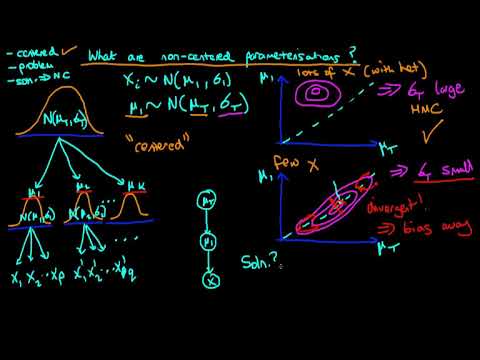
This is known as the centered parameterization. The geometry of the model can be tricky for gradient based MCMC and lead to divergent transitions. So sometimes a non-centered parameterization is needed. In this simple case, this can be done quite easily, though.

//lognormal_partial_pooling_ncp.stan
data {
  int<lower=1> N; //number of records
  int<lower=1> K; //number of groups (states)
  int<lower=1,upper=K> state[N]; //vector of state values
  real<lower=0> y[N]; //outcomes (loss amounts)
}
parameters {
  real mu0;
  real<lower=0> sigma0;
  vector<offset = mu0, multiplier = sigma0>[K] mu;
  real<lower=0> sigma;
}
model {
  //priors  
  mu0 ~ normal(9, 3);
  sigma0 ~ gamma(2, 1);
  mu ~ normal(mu0, sigma0);
  sigma ~ gamma(2, 1);
  //likelihood
  y ~ lognormal(mu[state], sigma);
}

Now, you’ll probably still get a few divergent transitions. You can crank up adapt_delta to something like 0.95 or even 0.99 to make them disappear. If they’re still there, there is probably something fishy in your model, or in your data.

First, I’d strong advise against just comparing posterior means. What you’d ideally want to do is simulate a bunch of data sets and see if the the 50% posterior interval contains the true parameter 50% of the time, the 75% interval contains it 75%, and so on.

Second, the way you’ve set up the unpooled model is not that great for the comparisons you want to make. This is how I set up the unpooled model:

//lognormal_unpooled.stan
data {
  int<lower=1> N; //number of records
  int<lower=1> K; //number of groups (states)
  int<lower=1,upper=K> state[N]; //vector of state values
  real<lower=0> y[N]; //outcomes (loss amounts)
}
parameters {
  real mu[K];
  real<lower=0> sigma;
}
model {
  //priors
  mu ~ normal(9, 3);
  sigma ~ gamma(2, 1);
  //likelihood
  y ~ lognormal(mu[state], sigma);
}

The obeservation-level sigma is fixed for all, and there is no sigma_0 that governs the amount of pooling. The mu’s come from an identical distribution, but don’t share any parameter (don’t share any information) compared to the partial pooling case.

Together with the pooled model

//lognormal_pooled.stan
data {
  int<lower=1> N; //number of records
  real<lower=0> y[N]; //outcomes (loss amounts)
}
parameters {
  real mu;
  real<lower=0> sigma;
}
model {
  //priors
  mu ~ normal(9, 3);
  sigma ~ gamma(2, 1);
  //likelihood
  y ~ lognormal(mu, sigma);
}

… I got these results (bars are 50% intervals, crosses are true values, dots are medians):
Rplot01
Note that I had to run the NCP (non-centered) model with adapt_delta = 0.95 to get rid of divergences. The centered parameterization always had divergences.

There are some implementations of the Tweedie distributions on here (more precisely the Compound Poisson Gamma part of the Tweedie). I’ll probably work on building a slightly more efficient version of it for my own work. Maybe that could be interesting to you in future?

Cheers!
Max

3 Likes

Thanks for the great response, Max! I am going to dig into this and will get back to you in the next few days. I’m interested in tweedie but first things first!

1 Like

Thanks again, Max. I’ve been reading through some Betancourt case studies and I’ve found them really helpful. The shinystan package if also handy, glad I saw that in one of the case studies.

The way you set up the partial pooling model makes sense to me now. I also couldn’t get rid of all divergences when playing around with it. I saw in one of the Betancourt case studies that a non-centered parameterization was used as well but I don’t really have a feel for what it’s doing, though, and why it alleviates the divergence issues. Even if I had correctly come up with the centered partial pooling model on my own, I would have never thought of the non-centered version. Do you have anything which helps explain the intuition behind it?

For your unpooled model, aren’t you pooling the \sigma parameter across states? I’m trying to set up my unpooled model to be the equivalent of taking each state’s data and running each through the pooled model, as if all 3 state’s parameters are estimated truly standalone. I should add that I’m not trying to produce estimates from the unpooled model, I’m more looking for the best way to demonstrate what hierarchical modeling is doing. I’m looking for a good numerical example to support the narrative around hierarchical modeling being a “credibility weighting” between pooled and unpooled estimates. To one of your other points, that is what drove me to focus on comparing mean estimates.

Thank you for this clear discussion both. I found it very helpful.

A bit late, but I found this video by Ben Lambert on non-centered parameterisation helped with my intuition:

3 Likes