Thank you for the kind advice and apologies for the broad framing of my question.
After reading some more I think I have narrowed in on what confuses me in this context.
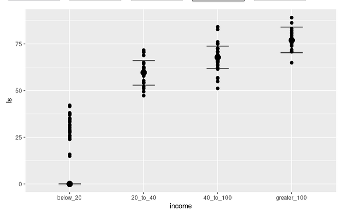
I ran some simulations using the same example given in the monotonic vignette and got the following results.
A) In a no intercept vs. with intercept model the first monotonic simplex parameter gets overestimated. Why is that? Is there a way to look at the design matrix used to fit the model? I saw the post and documentation about 0+ meaning not mean centering the predictors in the design matrix, but I don’t have a good intuition about what that means in the context of the monotonic function. In general I thought the 0+ syntax avoids computing the parameters with regards to a reference level of the categorical factor, but rather computes them with reference to the grand mean and the main problem in doing so is potential overparameterization. But now these simulations show different effect sizes for 1 of the parameters. I would have either expected the CI intervals to get bigger or the error estimate go up, but that does not seem to be the case.
income_options <- c("below_20", "20_to_40", "40_to_100", "greater_100")
income <- factor(sample(income_options, 100, TRUE),
                 levels = income_options, ordered = TRUE)
mean_ls <- c(30, 60, 70, 75)
ls <- mean_ls[income] + rnorm(100, sd = 7)
dat <- data.frame(income, ls)
fit1 <- brm(ls ~1 + mo(income), data = dat, seed = 123)


Formula: ls ~ 1 + mo(income)
   Data: dat (Number of observations: 100)
  Draws: 4 chains, each with iter = 2000; warmup = 1000; thin = 1;
         total post-warmup draws = 4000

Regression Coefficients:
          Estimate Est.Error l-95% CI u-95% CI Rhat Bulk_ESS Tail_ESS
Intercept    30.94      1.33    28.22    33.55 1.00     2862     2693
moincome     15.40      0.66    14.12    16.73 1.00     2757     2266

Monotonic Simplex Parameters:
             Estimate Est.Error l-95% CI u-95% CI Rhat Bulk_ESS Tail_ESS
moincome1[1]     0.63      0.04     0.56     0.71 1.00     3058     2049
moincome1[2]     0.17      0.04     0.08     0.25 1.00     3026     2253
moincome1[3]     0.20      0.04     0.12     0.28 1.00     3608     2327

Further Distributional Parameters:
      Estimate Est.Error l-95% CI u-95% CI Rhat Bulk_ESS Tail_ESS
sigma     6.86      0.50     5.95     7.91 1.00     3696     2570
fit2 <- brm(ls ~ 0 + mo(income), data = dat, seed = 123)


Formula: ls ~ 0 + mo(income)
   Data: dat (Number of observations: 100)
  Draws: 4 chains, each with iter = 2000; warmup = 1000; thin = 1;
         total post-warmup draws = 4000

Regression Coefficients:
         Estimate Est.Error l-95% CI u-95% CI Rhat Bulk_ESS Tail_ESS
moincome    25.66      1.17    23.42    28.01 1.00     2393     2559

Monotonic Simplex Parameters:
             Estimate Est.Error l-95% CI u-95% CI Rhat Bulk_ESS Tail_ESS
moincome1[1]     0.78      0.06     0.67     0.89 1.00     2354     1963
moincome1[2]     0.11      0.05     0.01     0.22 1.00     3311     2100
moincome1[3]     0.12      0.05     0.02     0.22 1.00     2614     1995

Further Distributional Parameters:
      Estimate Est.Error l-95% CI u-95% CI Rhat Bulk_ESS Tail_ESS
sigma    17.64      1.26    15.43    20.38 1.00     2545     2114
B) I also noted that the effect disappears when using the 0+ syntax in a non-linear model with an added categorical predictor. I don’t really understand how that makes a difference.
(Just the monotonic predictor in NL-syntax: larger effect is still there)
dat$x <- sample(c("a", "b", "c"), 100, TRUE)
fit7 <- brm(
 formula = bf(ls ~ 0 + inc,
              inc ~ 0 + mo(income),
              nl=TRUE),
 data = dat,
 seed = 123)


Formula: ls ~ inc
         inc ~ 0 + mo(income)
   Data: dat (Number of observations: 100)
  Draws: 4 chains, each with iter = 2000; warmup = 1000; thin = 1;
         total post-warmup draws = 4000

Regression Coefficients:
             Estimate Est.Error l-95% CI u-95% CI Rhat Bulk_ESS Tail_ESS
inc_moincome    25.66      1.17    23.42    28.01 1.00     2393     2559

Monotonic Simplex Parameters:
                 Estimate Est.Error l-95% CI u-95% CI Rhat Bulk_ESS Tail_ESS
inc_moincome1[1]     0.78      0.06     0.67     0.89 1.00     2354     1963
inc_moincome1[2]     0.11      0.05     0.01     0.22 1.00     3311     2100
inc_moincome1[3]     0.12      0.05     0.02     0.22 1.00     2614     1995

Further Distributional Parameters:
      Estimate Est.Error l-95% CI u-95% CI Rhat Bulk_ESS Tail_ESS
sigma    17.64      1.26    15.43    20.38 1.00     2545     2114
(monotonic predictor + categorical factor: Same results for monotonic predictor as with Intercept, despite specifying 0+ on both)
dat$x <- sample(c("a", "b", "c"), 100, TRUE)
fit6 <- brm(
 formula = bf(ls ~ 0 + inc + xvar,
              inc ~ 0 + mo(income),
              xvar ~ 0 + x,
              nl=TRUE),
 data = dat,
 seed = 123)


Formula: ls ~ 0 + inc + xvar
         inc ~ 0 + mo(income)
         xvar ~ 0 + x
   Data: dat (Number of observations: 100)
  Draws: 4 chains, each with iter = 2000; warmup = 1000; thin = 1;
         total post-warmup draws = 4000

Regression Coefficients:
             Estimate Est.Error l-95% CI u-95% CI Rhat Bulk_ESS Tail_ESS
xvar_xa         29.44      1.58    26.37    32.52 1.00     2445     2512
xvar_xb         31.82      1.79    28.27    35.33 1.00     2339     2529
xvar_xc         32.02      1.66    28.74    35.25 1.00     2436     2726
inc_moincome    15.21      0.69    13.85    16.56 1.00     2064     2375

Monotonic Simplex Parameters:
                 Estimate Est.Error l-95% CI u-95% CI Rhat Bulk_ESS Tail_ESS
inc_moincome1[1]     0.63      0.04     0.56     0.71 1.00     2788     2603
inc_moincome1[2]     0.17      0.04     0.08     0.25 1.00     2885     2230
inc_moincome1[3]     0.20      0.04     0.12     0.28 1.00     3278     2419

Further Distributional Parameters:
      Estimate Est.Error l-95% CI u-95% CI Rhat Bulk_ESS Tail_ESS
sigma     6.84      0.51     5.92     7.94 1.00     3208     2614
Sorry if these questions are still too basic for this forum, but I am also still new to statistical modeling as a whole. I would also take pointers to a more appropriate forum if they are out of place here.


