Dear all,
I am trying to model probability outcomes using a Beta likelihood with mean/precision parameterization.
Briefly on the data generating process:
I have several models that estimates the probability of a latent binary variable (using other data) and I am currently trying leverage the output of all the models/methods for a large number of events in a datasets (roughly 2k - 12k events in one dataset).
Unfortunately (with my current model setup), I’ve noticed a weird behavior for very small values where the mean is sometimes inferred to be larger than the largest observed value.
I.e., max(y_i)<\mu_i, for some set of observations y_i and their inferred mean \mu_i.
Here is my (current) model setup for the i:th event estimated by the j:th method:
\log(\mu^*_i)\sim\mathcal{N}^-(0, 5)\quad\quad\quad\quad\quad\quad\quad\;\;\,\text{//Means Prior}
\mu_i = 1 - \mu^*_i\quad\quad\quad\quad\quad\quad\quad\quad\quad\quad\;\;\quad\quad\quad\quad\text{//Means transform}
t_i\sim Logistic(\eta_i,\sigma_t)\quad\quad\quad\quad\quad\quad\quad\quad\quad\quad\quad\quad\quad\quad\;\;\text{//Precision priors}
\eta_i\sim\mathcal{N}(\mu_i^{-1},5)
\sigma_t\sim\exp(1)
y_{ij}\sim\beta(\mu_it_{i},(1-\mu_i)t_{i})\quad\quad\quad\quad\quad\quad\quad\quad\;\;\,\text{//Likelihood}
The choices for modeling the mean was so that smaller means would be closer to the largest prior density (as these are the ones that are problematic).
For the precision, I performed an approximation error analysis as follow:
- produce a range of means (\mu_i s) in (0,1).
- For each mean, start with some small precision (t_i).
- Draw a sample of {2, 3, 4, 5, 6} measurements from \beta(\mu t_i, (1-\mu_i)t_i).
- Calculate the sample mean and calculate the approximation error: 100*\left|1-\frac{\ bar{X}}{\mu_i}\right|.
- If error less than {1, 10, 50}% break, else do t_i\gets1.1*t_i and repeat 3-5.
Plotting the final precision against \mu_i was roughly linear on a log-log plot.
As such, I’ve tried a power-law regression on the precision using the mean (among a myriad of other things) but this only succeeded if the simulated data had a strong power-law dependency of the precision on the mean and did not generalize well on real data.
In fact, the mean estimate can sometimes be several magnitudes larger than the largest observed probability. I.e., sometimes the largest probability of a method could be 4*10^{-4} and the estimated mean 4*10^{-2}.
This issue seems to come from the fact that the precision also gets drastically underestimated for data with smaller means.
Here are example figures to illustrate the problem.
Comparing the sample mean with the mu parameter to simulate the data:
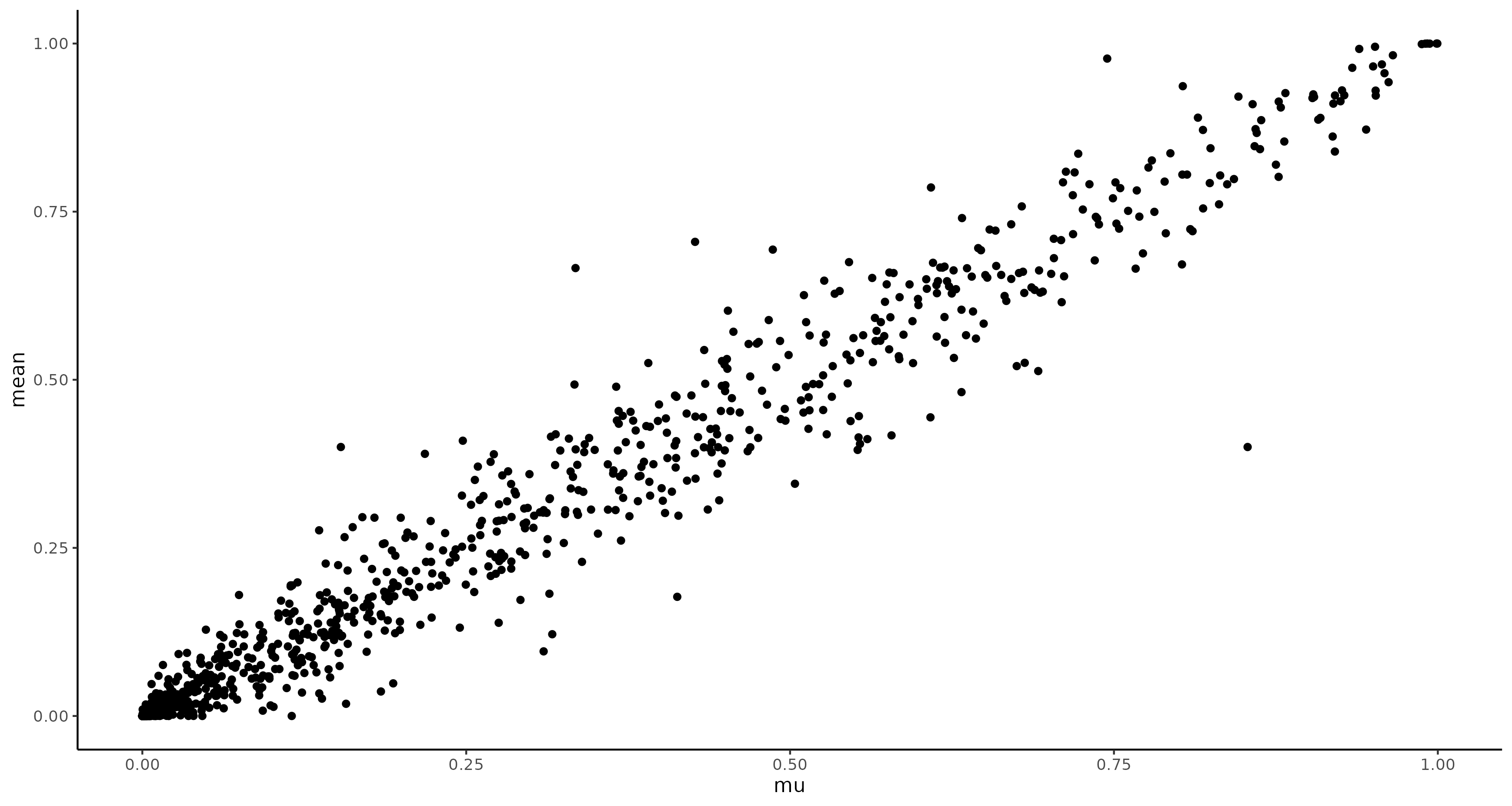
While when comparing the models inferred mean it produces strong underestimates for smaller means:

And here is just a table comparing the smallest inferred means with the real parameters:
# A tibble: 1,000 × 8
   index   eta     mu mu_star   t_i   mu_true ti_true mu_sample
   <int> <dbl>  <dbl>   <dbl> <dbl>     <dbl>   <dbl>     <dbl>
 1   981 0.798 0.0262   0.974  2.18 1.17e- 11   15.7  1   e-300
 2   666 0.793 0.0263   0.974  2.15 2.39e-  7    1.42 1   e-300
 3   229 0.832 0.0270   0.973  2.11 2.20e- 30    6.81 1   e-300
 4   402 0.823 0.0271   0.973  2.30 1   e-150   16.1  1   e-300
 5   933 0.811 0.0275   0.972  2.22 7.42e-  7    1.16 1   e-300
 6   151 0.798 0.0276   0.972  2.34 9.61e-  4    2.72 1.07e- 95
 7   140 0.812 0.0280   0.972  2.20 1.28e-  5   10.4  2.77e-148
 8    53 0.796 0.0283   0.972  2.31 4.99e-  7   10.4  1   e-300
 9   650 0.789 0.0284   0.972  2.33 1.74e-  4    6.29 6.54e- 43
10   540 0.767 0.0286   0.971  2.12 1.53e-  5   17.8  1   e-300
# ℹ 990 more rows
# ℹ Use `print(n = ...)` to see more rows
Where the smallest inferred mean is 0.03 while the true values is 1.17e-11 though some of these appear have been complete shrunk due to random chance (see random data generator at the end of post) as indicated by the sample mean.
Examining e.g., index 151 then this data is indeed much smaller than the inference:
[1] 7.728962e-238 1.957332e-272 5.335602e-95 5.915391e-115 5.434505e-276
Does anyone have any suggestions to setup this type of problem?
I’ve also tried a normal approximation for log(y) but it tends to have the same problems with overestimates.
Any suggestions are very welcomed!
Also, let me know if there is anything I can do to improve the post.
And here is the R code to reproduce the behavior with simulated data and the plots shown:
# Simulation function
beta_generator <- function(N, M = 5) {
  # Priors
  set.seed(1)
  # Ensure that each row gets roughly the same mean across simulations
  mu_dist <- rbeta(N, .5, 1.5)
  # Reset seed
  set.seed(NULL)
  # Mean precision
  mu_prec <- 1e1*mu_dist^-.005
  # Mean and precisions
  mu_i    <- rbeta(N, mu_prec*mu_dist, mu_prec*(1-mu_dist))
  t_i <- abs(rnorm(N, 1e1*mu_i^-.001, 5))
  # Likelihood
  y <- matrix(rbeta(N*M, mu_i*(t_i), (1 - mu_i)*(t_i)), N, M)
  # Avoid too large and too small values which causes log(0) error.
  y <- apply(y, c(1, 2), min, 1 - .Machine$double.eps*100000000)
  y <- apply(y, c(1, 2), max, 1e-300)
  # For running SBC
  list(
    variables = list(
      t_i = t_i,
      mu = mu_i
    ),
    generated = list(
      N = N, M = M, y = y
    )
  )
}
# Packages
require(pacman)
p_load(dplyr, tidyr, ggplot2, patchwork, cmdstanr)
# Sim data
sim_data <- beta_generator(1000)
# Produce stan inputs
stan_input <- list(
  N = sim_data$generated$N,
  M = sim_data$generated$M,
  y = sim_data$generated$y
)
# Stan model see end of post for model code
cmdstan_model <- cmdstanr::cmdstan_model("mwe_stan.stan")

# Fit the model
fit <- cmdstan_model$sample(stan_input, parallel_chains = 4, iter_warmup = 500, iter_sampling = 500)

# Get the inferred parameters
infered_pars <- fit$summary() %>%
  select(1, mean) %>%
  slice(-1:-2) %>%
  separate_wider_regex(variable, patterns = c("variable" = ".*", "\\[", "index" = "[0-9]*", "\\]")) %>%
  spread(variable, mean) %>%
  mutate(
    index = as.integer(index)
  ) %>%
  arrange(index) %>%
  mutate(
    mu_true = sim_data$variables$mu,
    ti_true = sim_data$variables$t_i,
    mu_sample = apply(sim_data$generated$y, 1, mean)
  ) %>%
  select(-mu_star)

# Plot them
infered_pars %>%
  ggplot(aes(mu, mu_true)) +
  geom_point() +
  theme_classic()
ggsave("mu_vs_mu_true.png")

p_sim <- infered_pars %>%
  ggplot(aes(mu, t_i)) +
  geom_point() +
  theme_classic()

p_true <- infered_pars %>%
  ggplot(aes(mu_true, ti_true)) +
  geom_point() +
  theme_classic()

p_sim + p_true
ggsave('prec_vs_mu.png')

# Table
infered_pars %>%
    arrange(mu)
data {
  int<lower=0> N;                      // Number of events
  int<lower=0> M;                      // Number of methods
  array[N, M] real<lower=0,upper=1> y; // Observed probabilities
}

parameters {
  real<lower=0> sl; // Precision variance
  vector<lower = 0>[N] eta; // Precision mean
  vector<lower = 0>[N] t_i; // Precision
  vector<lower = 0, upper = 1>[N] mu_star; // mu = 1 - mu_star
}
transformed parameters {
  vector<lower = 0, upper = 1>[N] mu = 1 - mu_star; // mean parameter
}
model {
  // Priors
  eta ~ std_normal();
  sl ~ exponential(1);
  t_i ~ logistic(eta, sl);
  for (i in 1:N) {
    real inv_log_mu = log(mu_star[i]);
    target += -inv_log_mu; // Jacobian
    inv_log_mu ~ normal(0, 5);
    // Likelihood
    y[i] ~ beta_proportion(mu[i], t_i[i]);
  }
}