Is higher adapt delta guaranteed to be higher possible successful estimation?

[steakdream]

I want to fit a panel MSVAR model through hierarchical prior setting.

I built my DGP for 3 regimes, 2 lags,
and I simulate the data with 3 units 2 variables and 20 time length(I know this is quite small).

I sample it by using warmup=2000, post iteration=1000, with 4 chains

The illustrate expression is like: y_{t} \sim A * y_{t-p} + (\mu_{1} \quad \text{or} \quad \mu_{2} \quad \text{or} \quad \mu_{3}),
, where A is the VAR part regime-invariate coefficients; “\mu_{m}”, m=1, 2, 3, are the mean of each state.
and the prior is: A, \mu_{m} \sim N(\mu_{A}/\mu_{mm}, 1), \mu_{A}/\mu_{mm} \sim N(0, 10), Covariance follows wishart.

I found that when
adapt delta=0.8, the highest Rhat of A is likely 1.003, lp__ is 1.01;
however, when I raise adapt delta to be higher, such as 0.99, the highest Rhat of A become 1.2, and the posterior draws of this coefficient will be like

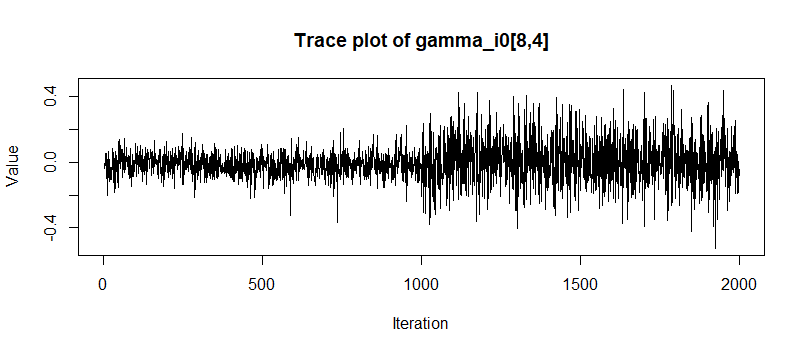
or multimodality.

I’m wondering that it seems that in the previous results and article, as long as we give enough max_treedeepth and warmup, higher adapt delta will likely result better convergence. But in my DGP, the best adapt delta is at the middle b/w 0.8-0.85, higher will result multimodality(I confirm it with up to 4 chains to avoid random seed luck; I also set max_treedepth=15 and there was no reporting of hitting), and lower will result divergent. I feel it is strange that if I give enough space of max_treedepth to traversal the likelihood(higher adapt delta and higher treedepth), it should always give the better result.

I am not sure that my DGP scenario is because of 1) low sample size, and it may be too small so that multiple solutions of VAR coefs have the same likelihood, similar to label switching. 2) NUTS’s feature? whose suitable adapt delta may indeed can be concave. 3) auto adjusted step size of NUTS is not that smart, 4) or something else?

[avehtari]

Higher adapt_delta leads to smaller adapted step sizes. The smaller step size lead to more accurate Hamiltonian dynamic sampling. If you don’t hit the maximum treedepth, there is no additional autocorrelation. As you observe multimodality with smaller step size, it indicates that your posterior really is multimodal, but with big enough step size, the probability of switching modes is so small that you don’t observe it with your current number of iterations (with infinite many iterations you would observe multimodality also with big step size).

[steakdream]

Hi, avehtari, nice to meet you again, and thanks for you relying.

I think that I found a coding strategy about HMM which will significantly affect the possibility to fit a HMM model successfully.

As what I specified previously, the panel MSVAR consists a regime-invariate VAR coef + regimes means(mu1 or mu2). The priors I used basically follow hierarchical structure of cov of 1 and 10,

\gamma_{i, 0/1/2} \sim N(\underline{\lambda}_{0/1/2}, 1), \underline{\lambda}_{0/1/2} \sim N(0, 10)
where subscript of 0 is the regime-invariate VAR coef; “1” is the mean of regime 1; “2” is the mean of regime 2, “i” is the panel unit.

=============background above=========================
When I was coding these regime 1 and 2’ means at the first time, I decleared them seperately, such as (noncenter in transformed parameters):

  array[N] vector[K] gamma_i1;
  array[N] vector[K] gamma_i2;
for (n in 1:N){
    gamma_i1[n] = lambda_m[1] + L_underline_Sigma_im[n, 1] * gamma_i1_raw[n];
    gamma_i2[n] = lambda_m[2] + L_underline_Sigma_im[n, 2] * gamma_i2_raw[n];
}

and other things like the means of VAR+regime and covariances, I still used array[N, M] declaration because I was trying to usearray[N] vector<lower=gamma_i1>[K] gamma_i2; to avoid label switching, but I gave up this restriction:

array[N, M] cholesky_factor_cov[K] L_covari;
array[N, T_eff, M] vector[K] mu_y;

where N is the number of units, K is the number of variables in the VAR system.
With 8 chains, for adapt_delta = 0.99, max_treedepth = 15 with 2k warmup and 1k iterations, the results are (where every 1k on the x-axis is one chain (8 chains in total)):

The highest Rhat of regime-invariate VAR coef \gamma_{i,0} is 1.00387 with ESS 4531.496 ,
lp__ has rhat=1.01, ess_bulk=1071.

However, with the same DGP, if I change the declaration to

array[N, M] vector[K] gamma_im;
for (m in 1:M){
  gamma_im[n, m] = lambda_m[m] + L_underline_Sigma_im[n, m] * gamma_im_raw[n, m];
}

and I modify the old gamma_i1[n] or gamma_i2[n] to gamma_im[n, 1] or gamma_im[n, 2], the posterior draws of lp__ is:

This version has the following results:
The highest Rhat of regime-invariate VAR coef \gamma_{i,0} is 1.02 with ESS 304.2151,
lp__ has rhat=1.11, ess_bulk=48.7.

Theoratically, I guess, given the same dataset, these two kinds of coding should have almost the same results I guess? But their posteriors seem to be totally different and especially lp__ appears multimodality in the later example.
From this point, I think stan must treat these two codes differently, do you have any clue why it happens? Is there any internal assumption of coding I’v ignored about the dependent parameters through array[N, M]?

Besides, I guess it is related to HMM’s regime specific parameters because I think in a simple OLS, scuh as y \sim \beta X, it is naturally to code \beta as a matrix instead of \beta_1, \beta_2,…etc., and if no, many ppl will notice this difference if it makes this large difference.

[Bob_Carpenter]

array[N] vector[K] gamma_i1;
array[N] vector[K] gamma_i2;
for (n in 1:N){
    gamma_i1[n] = lambda_m[1] + L_underline_Sigma_im[n, 1] * gamma_i1_raw[n];
    gamma_i2[n] = lambda_m[2] + L_underline_Sigma_im[n, 2] * gamma_i2_raw[n];
}

array[N, M] vector[K] gamma_im;
for (m in 1:M){
  gamma_im[n, m] = lambda_m[m] 
                   + L_underline_Sigma_im[n, m] * gamma_im_raw[n, m];
}

Without the rest of the context of the program, it’s not clear where n is getting defined here or how the second program relates to the first. If you want to convert to a single data structure, the easiest thing to do is tack the index on first and then copy the earlier definition

array[2, N] matrix[K] gamma_im;

for (n in 1:N) {
  gamma_im[1, n] = lambda_m[1] + L_underline_Sigma_im[n, 1] * gamma_i1_raw[n];
  gamma_im[2, n] = lambda_m[2] + L_underline_Sigma_im[n, 2] * gamma_i2_raw[n];
}

Then gamma_im[1] is equal to your old gamma_i1 and similarly for gamma_im[2] and gamma_i2. You can vectorize out the n as follows if everything’s declared to conform.

array[2, N] matrix[K] gamma_im;

gamma_im[1] = lambda_m[1] + L_underline_Sigma_im[ , 1]' * gamma_i1_raw;
gamma_im[2] = lambda_m[2] + L_underline_Sigma_im[ , 2]' * gamma_i2_raw;