Inappropriate parameter estimates in ordinal models

matti · January 14, 2021, 4:55pm

Hi,

There seems to be an issue with ordinal models whereby comparing two groups with identical data leads to non-zero estimates of effects on the latent mean and standard deviation.

Here’s a reproducible example using these two packages

library(tidyverse)
library(brms)

Here’s some example data, as you can see they are identical across groups

dat <- tribble(
  ~ID, ~Rating, ~Count,
  12,      1,     1,
  12,      2,     1,
  12,      3,     2,
  12,      4,     6,
  12,      5,    22,
  5,      1,     1,
  5,      2,     1,
  5,      3,     2,
  5,      4,     6,
  5,      5,    22
) %>% 
  mutate(ID = factor(ID))

I then estimate a pretty standard cumulative model where I allow the mean and variance of the latent variable to be different for the two groups. The only nonstandard thing here is using weights (so if I have massive data the model still runs fast) but it makes no difference here.

fit <- brm(
  bf(Rating | weights(Count) ~ 1 + ID) + lf(disc ~ 0 + ID , cmc=FALSE) ,
  family = cumulative("probit") ,
  data = dat,
)
summary(fit, prior = TRUE)

I would obviously expect effects on the mean and SD to be zero because the data are identical, but here are the results:

 Family: cumulative 
  Links: mu = probit; disc = log 
Formula: Rating | weights(Count) ~ 1 + ID 
         disc ~ 0 + ID
   Data: dat (Number of observations: 10) 
Samples: 4 chains, each with iter = 2000; warmup = 1000; thin = 1;
         total post-warmup samples = 4000

Priors: 
Intercept ~ student_t(3, 0, 2.5)

Population-Level Effects: 
             Estimate Est.Error l-95% CI u-95% CI Rhat Bulk_ESS Tail_ESS
Intercept[1]    -2.12      0.43    -3.09    -1.36 1.00     1866     2272
Intercept[2]    -1.64      0.33    -2.33    -1.02 1.00     2754     2940
Intercept[3]    -1.17      0.26    -1.71    -0.68 1.00     4355     2995
Intercept[4]    -0.43      0.23    -0.88     0.02 1.00     3939     3618
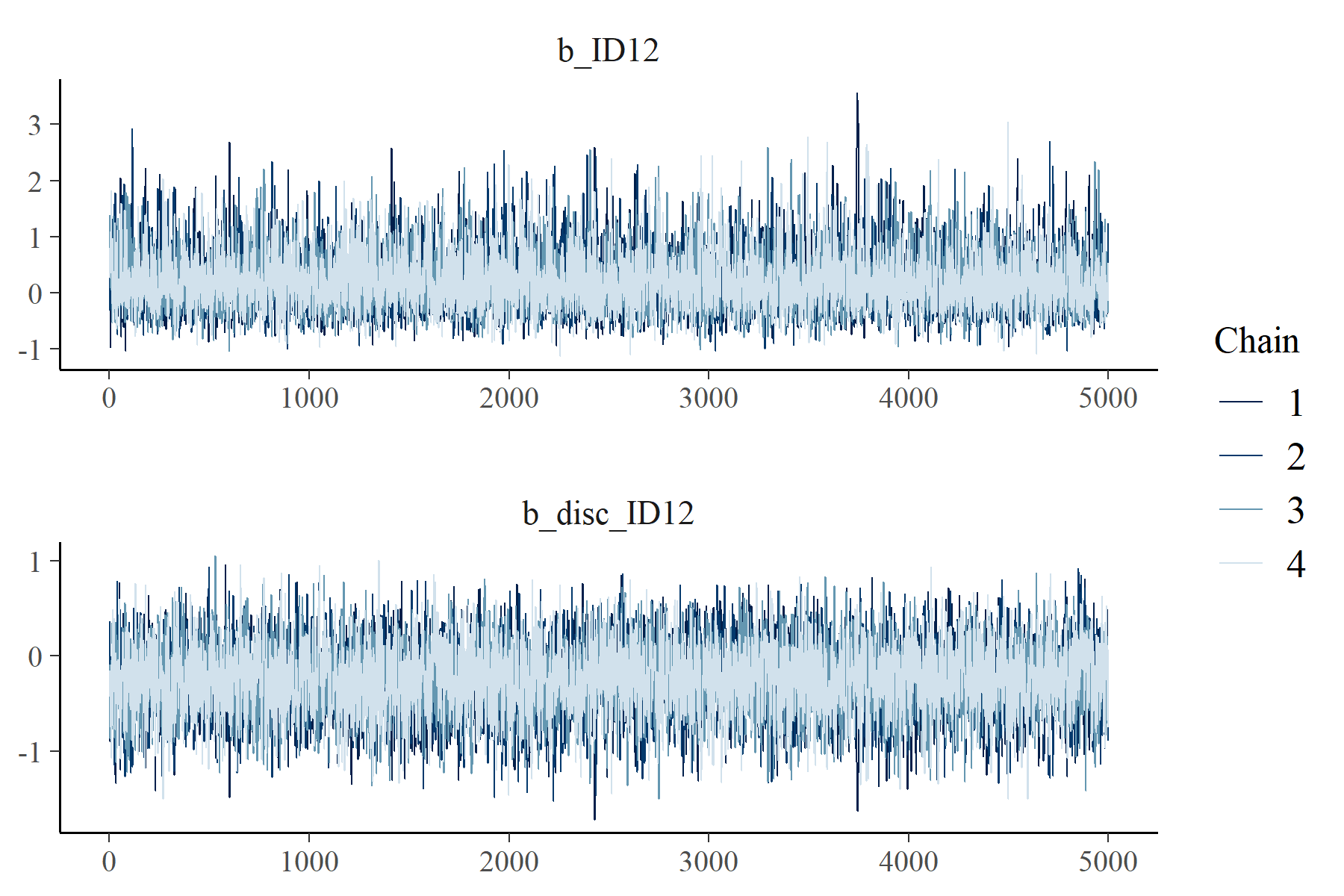
ID12             0.25      0.53    -0.57     1.52 1.00     1426     1598
disc_ID12       -0.25      0.37    -0.98     0.47 1.00     1192     1970

Samples were drawn using sampling(NUTS). For each parameter, Bulk_ESS
and Tail_ESS are effective sample size measures, and Rhat is the potential
scale reduction factor on split chains (at convergence, Rhat = 1).

This is pretty surprising behaviour (to me at least). I talked about it with @paul.buerkner (who probably has a thing or two to say about it), but if anyone else has insight into why this is happening, I’m all ears. Thanks!

mike-lawrence · January 14, 2021, 10:00pm

Which row(s) in the summary stick out as unexpected? If I understand correctly, the four intercept columns are showing the expected ordered relationship, and the remaining two have wide intervals that are consistent with zero.

paul.buerkner · January 14, 2021, 10:07pm

But they should be exactly zero based on the symmetry of the data. At least in the absence of prior information.

mike-lawrence · January 14, 2021, 10:08pm

Ahh, that makes sense. Could warmup not be resolving well, leaving things susceptible to the random init values?

matti · January 15, 2021, 9:37am

Thanks for the suggestion, but that’s almost certainly not the case. To verify I ran with 5000 warmup and subsequent 5000 iterations and results are the same:

The chains mix well and there is nothing in the diagnostics to indicate poor sampling.

However, if we change the situation a bit and assume that we have 50x more observations, the model behaves much better:

fit <- brm(
  bf(Rating | weights(Count) ~ 1 + ID) + 
    lf(disc ~ 0 + ID, cmc=FALSE),
  family = cumulative("probit"),
  data = dat %>% mutate(Count = Count * 50),
  warmup = 5000, iter = 10000
)
summary(fit, prior = TRUE)

 Family: cumulative 
  Links: mu = probit; disc = log 
Formula: Rating | weights(Count) ~ 1 + ID 
         disc ~ 0 + ID
   Data: dat %>% mutate(Count = Count * 50) (Number of observations: 10) 
Samples: 4 chains, each with iter = 10000; warmup = 5000; thin = 1;
         total post-warmup samples = 20000

Priors: 
Intercept ~ student_t(3, 0, 2.5)

Population-Level Effects: 
             Estimate Est.Error l-95% CI u-95% CI Rhat Bulk_ESS Tail_ESS
Intercept[1]    -1.87      0.06    -1.99    -1.75 1.00     9127    11262
Intercept[2]    -1.54      0.05    -1.63    -1.45 1.00    11679    13696
Intercept[3]    -1.15      0.04    -1.22    -1.08 1.00    19135    16185
Intercept[4]    -0.49      0.03    -0.55    -0.42 1.00    19276    17095
ID12             0.01      0.06    -0.11     0.13 1.00     9570    11647
disc_ID12       -0.01      0.06    -0.12     0.11 1.00     7599    10557

Samples were drawn using sampling(NUTS). For each parameter, Bulk_ESS
and Tail_ESS are effective sample size measures, and Rhat is the potential
scale reduction factor on split chains (at convergence, Rhat = 1).

Max_Mantei · January 15, 2021, 11:24am

Hey!

Could it be that the model is just not that well identified? Estimating both parameters of the latent variable and having just one restriction on the cut points would result in an unidentified model, right? In this case you estimate the latent sd only for one group, which might be the reason that the model does not fail.

bayesplot::mcmc_pairs(fit, regex_pars = "ID")

The solution is either more data or more informative priors. You already showed that more data helps and in the small data case you can see how imposing, for example, set_prior("normal(0, 0.25)", coef = "ID12", dpar = "disc"), can also help. (Note that this also pushes the latent mean estimate of the difference in the correct direction.)

I could be wrong, though!

Cheers,
Max

matti · January 18, 2021, 3:53pm

Hi @Max_Mantei, thanks for your input. I am not sure if that is the reason because I can estimate the same model using maximum likelihood, without problems, as implemented in the ordinal package:

library(ordinal)
x <- clm(
  ordered(Rating) ~ ID, ~ID, 
  data = dat, 
  weights = Count, 
  link = "probit"
)
summary(x)
formula: ordered(Rating) ~ ID
scale:   ~ID
data:    dat

 link   threshold nobs logLik AIC    niter max.grad cond.H 
 probit flexible  64   -61.53 135.06 5(1)  1.25e-08 3.6e+01

Coefficients:
      Estimate Std. Error z value Pr(>|z|)
ID12 -3.22e-10   4.33e-01       0        1

log-scale coefficients:
      Estimate Std. Error z value Pr(>|z|)
ID12 -4.28e-10   4.03e-01       0        1

Threshold coefficients:
    Estimate Std. Error z value
1|2   -1.863      0.411   -4.53
2|3   -1.534      0.330   -4.65
3|4   -1.150      0.266   -4.33
4|5   -0.489      0.231   -2.11

Both ID coefficients are exactly zero, as one would expect given identical data for the two groups.

mike-lawrence · January 18, 2021, 4:52pm

Does the observed behaviour remain consistent across different init seeds?

paul.buerkner · January 18, 2021, 7:59pm

Does the observed behaviour remain consistent across different init seeds?

In my tests, yes.

MilaniC · January 19, 2021, 3:36am

@matti

Your ordinal::clm() model enforces an implicit intercept for the scale component but you excluded it from your brms::brm() model.

Putting the intercept back into lf(...) for the brms::brm() model, with cmc=TRUE (or FALSE) and adequate iterations, does yield zeros (presumably relative to the estimated scale intercept).

It seems to me that the specified ordinal::clm() model is not consistent with the specified brms::brm() model and perhaps why you get expected estimates with the former and not the latter.

Maybe that is the issue?

matti · January 25, 2021, 5:02pm

Thanks @MilaniC! I wasn’t aware that ordinal::clm() has an implicit intercept for the scale. Would that mean that in this example the scale parameter is estimated for both groups? Because if you do that explicitly by

x <- clm(
  ordered(Rating) ~ ID, ~ 0 + ID, 
  data = dat, 
  weights = Count, 
  link = "probit"
)
summary(x)

you get NAs for the second group’s scale coefficient:

formula: ordered(Rating) ~ ID
scale:   ~0 + ID
data:    dat

 link   threshold nobs logLik AIC    niter max.grad cond.H 
 probit flexible  64   -61.53 135.06 5(1)  1.25e-08 1.1e+02

Coefficients:
      Estimate Std. Error z value Pr(>|z|)
ID12 3.223e-10  4.328e-01       0        1

log-scale coefficients: (1 not defined because of singularities)
       Estimate Std. Error z value Pr(>|z|)
ID5  -4.276e-10  4.027e-01       0        1
ID12         NA         NA      NA       NA

Threshold coefficients:
    Estimate Std. Error z value
1|2  -1.8627     0.6299  -2.957
2|3  -1.5341     0.5445  -2.817
3|4  -1.1503     0.4595  -2.504
4|5  -0.4888     0.3364  -1.453

Thanks!
Matti

Topic		Replies	Views
Question about family = cumulative in brms Modeling ordinal-response , priors , brms	5	1208	April 4, 2023
Multilevel ordinal model - large values in threshold and group level sd estimates? brms brms	2	570	May 3, 2021
Using brm to reproduce analysis of Liddell and Kruschke (2018) brms ordinal-response	3	360	February 5, 2024
Brms: how can I compare differences of variance of marginal_effects() for categories (i.e. category probabilities) brms techniques	4	528	September 1, 2020
Problem running mixed effect model with ordinal outcome and ordinal predictors with brms brms	2	1656	April 9, 2019

Inappropriate parameter estimates in ordinal models

Related Topics