Improving efficiency of a multilevel binomial logit model

Hi all,

I’m hoping to get some pointers that might improve sampling efficiency for a multilevel, binomial logit model I’ve been working on. The current version of the model (below) appears to fit the data well according to comparisons of the ‘n_successes’ observed and the ‘y_new’ detailed in the generated quantities block below. Likewise, the parameters fit closely resemble patterns from a log-normal version of the model I’ve fit previously. In that model, someone else had generated estimates for log-concentrations derived from the raw binomial data. This is digital PCR data.

Here, of course, I’m looking to fit the raw, binomial data; however, the model takes around an hour and a half to fit the N=1850 observations. This is compared to about a minute or less for the log-normal version. Likewise, the sampling appears to less than ideal. Here is a summary from the last run (sorry for formatting: pointers accepted):

Inference for Stan model: stan-45e01a247373.
4 chains, each with iter=1000; warmup=500; thin=1;
post-warmup draws per chain=500, total post-warmup draws=2000.

            mean se_mean    sd     2.5%      25%      50%      75%    97.5% n_eff Rhat
b0            -6.84    0.02  0.29    -7.40    -7.03    -6.84    -6.65    -6.28   173 1.02
b1             1.98    0.03  0.24     1.51     1.82     1.97     2.14     2.47    67 1.05
sigma          2.19    0.00  0.04     2.11     2.16     2.18     2.21     2.27    93 1.03
sigma_a[1]     1.36    0.01  0.20     1.02     1.22     1.34     1.48     1.81   255 1.01
sigma_a[2]     0.64    0.02  0.24     0.16     0.49     0.64     0.80     1.15    98 1.02
Omega[1,1]     1.00    0.00  0.00     1.00     1.00     1.00     1.00     1.00  2000  NaN
Omega[1,2]    -0.29    0.02  0.26    -0.74    -0.47    -0.30    -0.12     0.24   272 1.00
Omega[2,1]    -0.29    0.02  0.26    -0.74    -0.47    -0.30    -0.12     0.24   272 1.00
Omega[2,2]     1.00    0.00  0.00     1.00     1.00     1.00     1.00     1.00  1995 1.00
lp__       -6473.63    3.99 41.23 -6553.38 -6502.59 -6473.49 -6446.74 -6394.12   107 1.03

Samples were drawn using NUTS(diag_e) at Tue May 22 13:38:43 2018.
For each parameter, n_eff is a crude measure of effective sample size,
and Rhat is the potential scale reduction factor on split chains (at
convergence, Rhat=1).

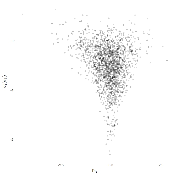
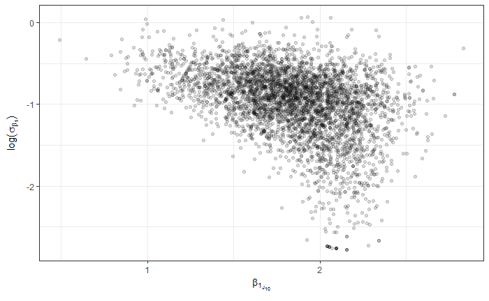
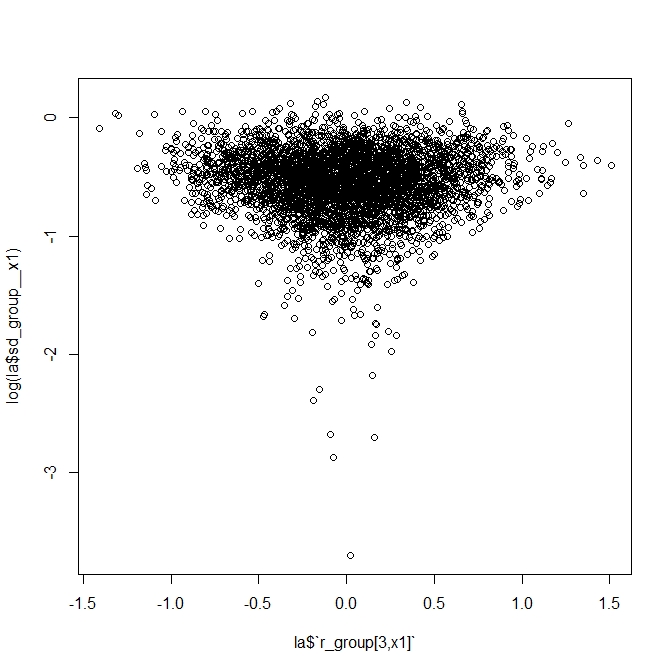
So, all in all, I was hoping maybe I’m missing something with the parameterization or coding that might help me improve the efficiency. I’ll note that the data might be characterized as high N and low p, in the context of Bin( N, p ). For example, the median n_trials is around 16000 and median n_success around 30. So, for p, the vast majority of obs should be much less than p=0.1, but with a few obs as high as 0.8. I’m thinking this is maybe where I’m getting into trouble, but I thought I’d post here to see if there are any glaring errors or other obvious areas for improvement.

Many thanks,

-Roy

Code below:

data{
 int<lower=1> N;  // number of observations
 int<lower=0> y[N];  // n success
 int<lower=1> n[N];  // n trials
 int<lower=1> J;  // n groups
 vector[N] x1;  // covariate vector: 0/1
 int<lower=1, upper=J> group[N];  // indexing J groups to N obs
 vector<lower=0>[N] sample_vol;  // volume of sample (mL) for gen. quant.
 }
parameters{
 real b0;  // sample-level mean of success (log-odds)
 real b1;  // sample-level covariate slope
 vector[N] eps_z; 
 matrix[2, J] a_z; 
 real<lower=0> sigma_z; 
 vector<lower=0>[2] sigma_a_z; 
 cholesky_factor_corr[2] L_Omega_J;
 }
transformed parameters {
 vector[N] p_logit;  // success (log-odds)
 vector[N] eps;  // sample-level error term: eps ~ N(0, sigma)
 matrix[J, 2] a;  // group-level slopes and intercepts matrix: cbind( \alpha_J , \beta_{1_J} )
 vector[J] a_J;  // group-level intercepts: \alpha_J
 vector[J] b1_J;  // group-level slopes: \beta_{1_J}
 real<lower=0> sigma;  // sample-level sd
 vector<lower=0>[2] sigma_a;  // group-level sds for intercepts and slopes
 cholesky_factor_cov[2] L_Sigma_J;  // Chol. cov. matrix for slopes and intercepts
 
 {
  sigma = sigma_z * 5; // scaling prior sd
  eps = eps_z * sigma;  // scaling error term
  sigma_a[1] = sigma_a_z[1] * 3; // scale prior for intercepts
  sigma_a[2] = sigma_a_z[2] * 3; // scale prior for slopes
  
  L_Sigma_J = diag_pre_multiply(sigma_a, L_Omega_J); 
  a = (L_Sigma_J * a_z)';
  a_J = col(a, 1);
  b1_J = col(a, 2);
 
  for (i in 1:N){
   p_logit[i] = ( b0 + ( ( b1 + b1_J[group[i]] ) * x1[i] ) + eps[i] ) + a_J[group[i]];
   }
  }
 }
model{
 b0 ~ normal( -5 , 3 );
 b1 ~ normal( 0 , 5 );
 
 eps_z ~ normal( 0 , 1 );
 to_vector(a_z) ~ normal( 0 , 1 );
 
 sigma_z ~ normal( 0 , 1 ); 
 sigma_a_z[1] ~ normal( 0 , 1 ); // \sigma_{\alpha_J}
 sigma_a_z[2] ~ normal( 0 , 1 ); // \sigma_{\beta_{1_J}}
 L_Omega_J ~ lkj_corr_cholesky(4);
 
 {
  target += binomial_logit_lpmf( y | n , p_logit );
  }
 }
generated quantities{
 real p_hat[N];
 real conc_hat[N];
 real y_hat[N];
 real y_new[N];
 real conc_new[N];
 matrix[2, 2] Omega;
 {
  Omega = multiply_lower_tri_self_transpose(L_Omega_J);
  
  for ( i in 1:N ) {
   p_hat[i] = inv_logit( p_logit[i] );
   y_hat[i] = p_hat[i] * n[i];
   conc_hat[i] = ( -log( 1 - ( y_hat[i] / n[i] ) ) / 0.00085 ) * ( 1500 / sample_vol[i] );
   y_new[i] = binomial_rng( n[i] , p_hat[i] );
   conc_new[i] = ( -log( 1 - ( y_new[i] / n[i] ) ) / 0.00085 ) * ( 1500 / sample_vol[i] );
   }
  }
 }

Hi again, and sorry for the apparent lack of information in the OP. I wanted to update the post, however, to note that I believe I tracked down the offending ‘funnel’, which appears to show that the ‘random slopes’ were a problem area. To reference the code, there appears to be a textbook funnel in the scatterplot of posteriors for log(sigma_a[2]) vs. b1_J, which is a plot of log-scale sd of the slopes vs. any given slope b1_J.

log_sigma_B1_v_B1_J

With that in mind, I created a sim for the model in R, and I found that, although the Stan model in the OP recovered the parameters and was funnel-free for most simulated realizations of the parameters, the fit got complicated (i.e., funnels) when I set the parameters in the sim to those suggested by the original fit to my data (i.e., ‘print’ in OP), which are maybe fairly extreme with b0, or mean success (log-odds) near -7 and sd (sigma) near 2; and particularly when the standard deviation in slopes was relatively small (around 0.6 in this case).

In the end, I did find a parameterization that appeared to work much better, though there is still the semblance of a funnel there:

log_sigma_B1_vs_B1_10

Nevertheless I think this was maybe one of those issues where the centered was much better than non-centered. For reference, the data were N=1850 or so observations from J=27 groups.

Inference for Stan model: stan-50b8e2e436d.
4 chains, each with iter=2000; warmup=1000; thin=1;
post-warmup draws per chain=1000, total post-warmup draws=4000.

            mean se_mean   sd  2.5%   25%   50%   75% 97.5% n_eff Rhat
b0         -7.08    0.00 0.28 -7.61 -7.27 -7.08 -6.90 -6.54  4000 1.00
b1          2.16    0.00 0.13  1.90  2.08  2.16  2.25  2.40  2738 1.00
sigma       1.95    0.00 0.04  1.88  1.92  1.95  1.97  2.02  4000 1.00
sigma_a[1]  1.38    0.00 0.22  1.02  1.23  1.36  1.51  1.89  4000 1.00
sigma_a[2]  0.41    0.01 0.15  0.12  0.31  0.41  0.51  0.73   433 1.01
Omega[1,1]  1.00    0.00 0.00  1.00  1.00  1.00  1.00  1.00  4000  NaN
Omega[1,2]  0.20    0.01 0.24 -0.27  0.04  0.21  0.37  0.64  2049 1.00
Omega[2,1]  0.20    0.01 0.24 -0.27  0.04  0.21  0.37  0.64  2049 1.00
Omega[2,2]  1.00    0.00 0.00  1.00  1.00  1.00  1.00  1.00  4000 1.00

Samples were drawn using NUTS(diag_e) at Thu May 31 14:33:55 2018.
For each parameter, n_eff is a crude measure of effective sample size,
and Rhat is the potential scale reduction factor on split chains (at 
convergence, Rhat=1).

Below is the code for the sim and revised Stan model, in case anyone is interested:

#library(rstan)
#library(rethinking)
#library(truncnorm)
#options(mc.cores = parallel::detectCores())
#rstan_options(auto_write = TRUE)

N <- 1850 #observations
J <- 27 #groups
x1 <- rbinom(n=N, size=1, prob= 0.5) #covariate
n <- rpois(n=N, lambda=16000) #randomly generate n_trials
group <- sample(1:J, size=N, replace=TRUE) #generate group index

b0 <- -6.5 #rnorm(1, -5, 3) #sample-level mean of success (log-odds)
b1 <- 2 #rnorm(1, 0, 3) #sample-level covariate effect
sigma <- 2 #rtruncnorm(n=1, a=0, b=Inf, mean=0, sd=3) #sample-level sd
sigma_a_J <- 1.5 #rtruncnorm(n=1, a=0, b=Inf, mean=0, sd=3) #group intercepts sd
sigma_B1_J <- 0.5 #rtruncnorm(n=1, a=0, b=Inf, mean=0, sd=3) #group slopes sd

eps <- rnorm(N, 0, sigma) #sample-level error term

Omega_J <- rlkjcorr(n=1, K=2, eta=2) #generate random corr matrix
Sigma_J <- diag(c(sigma_a_J,sigma_B1_J)) %*% Omega_J %*% diag(c(sigma_a_J,sigma_B1_J)) #convert to covariance
L_Sigma_J <- t(chol(Sigma_J)) #Lower Cholesky

a <- t(L_Sigma_J %*% matrix(rnorm(J*2, 0, 1),2,J)) #matrix of random effects
a_J <- a[,1] #random intercepts
b1_J <- a[,2] #random slopes
rm(a)

mu_p_logit <- rep(NA, N) #container for loop
for (i in 1:N){
 mu_p_logit[i] <- ( b0 + ( ( b1 + b1_J[group[i]] ) * x1[i] ) + eps[i] ) + a_J[group[i]]
 }

y <- rep(NA, N) #container for y or n_successes
for (i in 1:N){
  y[i] <- rbinom(n=1, size=n[i], prob=inv_logit(mu_p_logit[i]))
}

#make data list for Stan
stan_dataList <- list(N=N,
                      y=y,
                      n=n,
                      J=J,
                      x1=x1,
                      group=group,
                      sample_vol=rep(50, N)
                      )
data{
 int<lower=1> N;  // number of observations
 int<lower=0> y[N];  // n success
 int<lower=1> n[N];  // n trials
 int<lower=1> J;  // n groups
 vector[N] x1;  // covariate vector: 0/1
 int<lower=1, upper=J> group[N];  // indexing J groups to N obs
 vector<lower=0>[N] sample_vol;  // volume of sample (mL) for gen. quant.
 }
parameters{
 vector[N] p_logit;  // success (log-odds)
 real b0;  // sample-level mean of success (log-odds)
 real b1;  // sample-level covariate slope
 matrix[J, 2] a; // group-level slopes and intercepts matrix: cbind( \alpha_J , \beta_{1_J} )
 real<lower=0> sigma; // sample-level sd
 vector<lower=0>[2] sigma_a; 
 cholesky_factor_corr[2] L_Omega_J;
 }
transformed parameters {
 vector[J] a_J;  // group-level intercepts: \alpha_J
 vector[J] b1_J;  // group-level slopes: \beta_{1_J}
 cholesky_factor_cov[2] L_Sigma_J;  // Chol. cov. matrix for slopes and intercepts
 
 L_Sigma_J = diag_pre_multiply(sigma_a, L_Omega_J); 
 a_J = col(a, 1);
 b1_J = col(a, 2);
 }
model{
 b0 ~ normal( -5 , 3 );
 b1 ~ normal( 0 , 5 );
 sigma ~ normal( 0 , 3 );
 sigma_a[1] ~ normal( 0 , 3 ); // \sigma_{\alpha_J}
 sigma_a[2] ~ normal( 0 , 3 ); // \sigma_{\beta_{1_J}}
 L_Omega_J ~ lkj_corr_cholesky(4);
 {
  vector[2] ab;
  ab[1] = b0;
  ab[2] = b1;
  
  for (j in 1:J){
   a[j,] ~ multi_normal_cholesky( ab , L_Sigma_J );
   }
   
  for (i in 1:N){
   p_logit[i] ~ normal( a_J[group[i]] + ( b1_J[group[i]] * x1[i] ) , sigma );
   }
   
  target += binomial_logit_lpmf( y | n , p_logit );
  }
 }
generated quantities{
 real p_hat[N];
 real conc_hat[N];
 real y_hat[N];
 real y_new[N];
 real conc_new[N];
 matrix[2, 2] Omega;
 {
  Omega = multiply_lower_tri_self_transpose(L_Omega_J);
  
  for ( i in 1:N ) {
   p_hat[i] = inv_logit( p_logit[i] );
   y_hat[i] = p_hat[i] * n[i];
   conc_hat[i] = ( -log( 1 - ( y_hat[i] / n[i] ) ) / 0.00085 ) * ( 1500 / sample_vol[i] );
   y_new[i] = binomial_rng( n[i] , p_hat[i] );
   conc_new[i] = ( -log( 1 - ( y_new[i] / n[i] ) ) / 0.00085 ) * ( 1500 / sample_vol[i] );
   }
  }
 }
2 Likes

Out of interest, if you let the brms R package generate and fit the Stan model, how does it perform as compared to your custom code?

1 Like

Hi Paul,

Sorry for delayed response, it took me while to get around to your proposal. I’m also not that familiar with brms, so it took me a bit to learn enough in to be able to cobble a model together.

Using brms, I tried this model on data simulated using the same R code and parameter settings as above:

brms_dat <- data.frame(cbind(stan_dataList$y,
                             stan_dataList$n,
                             stan_dataList$x1,
                             ind=seq(1, length(stan_dataList$y),1),
                             stan_dataList$group))

colnames(brms_dat) <- c("y","n","x1","ind","group")


mbl_brms <- brm( y | trials(n) ~ x1 + (1 + x1 | group) + (1 | ind) ,
                 data=brms_dat, 
                 family=binomial(link="logit"),
                 prior=c(set_prior("normal(0,3)", class="b", coef="x1"),
                         set_prior("normal(0,3)", class="sd"),
                         set_prior("lkj(4)", class="cor")
                         ),
                         warmup=500,
                         iter=1000,
                         control=list(adapt_delta=0.90,
                                      max_treedepth=14)
                         )

It definitely took a longer to run than the custom versions I tried, though admittedly it is likely I may have messed something up with the brms model statement. I ended up letting it run overnight to finish, as warmup alone was around 5200s. Because the pc went to sleep or something in the middle of the night, and started back up after I woke it the next morning, it was hard to know exactly how long it should have taken. Nevertheless, here are some relevant findings:

First I got the warning:

Compiling the C++ model
Start sampling
Loading required namespace: rstudioapi
There were 3502 transitions after warmup that exceeded the maximum treedepth. Increase max_treedepth 
above 12. See
http://mc-stan.org/misc/warnings.html#maximum-treedepth-exceededExamine the pairs() plot to diagnose 
sampling problems

This was also a problem with some earlier attempts with my custom models, so I should have thought to increase the max_treedepth a bit more.

Parameter recovery was OK, as in the other models, but, again, n_eff was pretty low all around:

  Family: binomial 
  Links: mu = logit 
Formula: y | trials(n) ~ x1 + (1 + x1 | group) + (1 | ind) 
   Data: brms_dat (Number of observations: 1850) 
Samples: 4 chains, each with iter = 2000; warmup = 1000; thin = 1;
         total post-warmup samples = 4000

Group-Level Effects: 
~group (Number of levels: 30) 
                  Estimate Est.Error l-95% CI u-95% CI Eff.Sample Rhat
sd(Intercept)         2.82      0.38     2.20     3.72        845 1.00
sd(x1)                0.60      0.15     0.31     0.90        103 1.02
cor(Intercept,x1)    -0.22      0.20    -0.59     0.20        552 1.00

~ind (Number of levels: 1850) 
              Estimate Est.Error l-95% CI u-95% CI Eff.Sample Rhat
sd(Intercept)     2.09      0.04     2.02     2.16        381 1.00

Population-Level Effects: 
          Estimate Est.Error l-95% CI u-95% CI Eff.Sample Rhat
Intercept    -5.57      0.51    -6.59    -4.58        318 1.02
x1            1.92      0.15     1.63     2.22        460 1.01

Samples were drawn using sampling(NUTS). For each parameter, Eff.Sample 
is a crude measure of effective sample size, and Rhat is the potential 
scale reduction factor on split chains (at convergence, Rhat = 1).

Overall, it did seem to improve maybe a little on the funnel, but as you can see in the figure, there is still some semblance there.

In any case, thanks for the suggestion. It was interesting to peruse the capabilities of brms via the various documentation and vignettes; and I hope to dig a little more into that in the future.

Thanks again,

-Roy