Hello,
To answer your question in a more general way, the easiest thing to do here would be to get prior predictive distributions. You could run your model without adding data and thereby simply get your priors back. This would show you what you are implying for each parameter.
To show you what I mean I’ll give the following example:
library(rstan)
m <- '
data{
 int<lower = 0> n;
 real y[n];
 int<lower = 0, upper = 1> run_estimation;
}

parameters {
 real m;
 real<lower = 0> v;
}

transformed parameters {
 real s;
 s = sqrt(v);
}

model {
 m ~ normal(0, 1);
 s ~ normal(0, 1);

 if(run_estimation){
  y ~ normal(m, s);
 }

}

'

sm <- stan_model(model_code = m)
set.seed(123)
y <- rnorm(100, 2, 3)
fit <- sampling(sm, data = list(y = y,
                                n = 100,
                                run_estimation = 0),
                seed = 1)
bayesplot::mcmc_dens(fit, pars = c("m", "s", "v"))
If you run the above code you find the following plot:
From this you find that the standard normal distribution that you specified on m is nicely showing up. As is the half normal on s. In addition we also find what the prior about v is. We did not specify anything directly concerning it, but we find what we indirectly implied about this parameter.
We could also omit any specification of priors and do this and we find out what the implicit priors are. In this case we run into some trouble and we would get all sorts of warnings, this table:
               mean se_mean            sd           2.5%            25%            50%           75%         97.5% n_eff Rhat
m     -1.617400e+03  671.55  2.178700e+03  -6.197020e+03  -3.213920e+03  -1.415470e+03  1.178000e+01  1.981910e+03    11 1.52
v     8.982657e+307     NaN           Inf  3.687373e+306  4.298573e+307  8.906685e+307 1.369914e+308 1.769636e+308   NaN  NaN
s     8.903230e+153     NaN 3.249876e+153  1.920253e+153  6.556348e+153  9.437524e+153 1.170433e+154 1.330277e+154   NaN 1.00
lp__   7.087600e+02    0.06  1.050000e+00   7.059000e+02   7.083500e+02   7.090800e+02  7.095100e+02  7.097700e+02   358 1.00
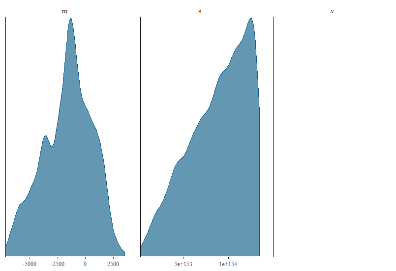
and this figure:
We see that we run into problems. Why? And now to anser your question more directly I quote from the stan prior choice wiki:
... you could just specify no prior at all, which in Stan is equivalent to a noninformative uniform prior on the parameter.
If you have constraints on the parameter, e.g. it is a correlation which can be between -1 and 1, these constraints are taken into account, if I am correct, and a uniform prior will be specified on the parameter space given those constraints.
Hope this helps,
Best, Duco