"Hypothesis testing" with multi-level models (for a Registered Report)

[Alasdair_Clarke]

Hello,

I am helping a friend with a Registered Report (a paper format inwhich your introduction + methods are peer reviewed before you conduct the experiment). As part of this, we’re working out our decision criteria and processes ahead of time. Luckily, for the sample size justification we have some related data from an earlier study.

The experiment is relatively simple: participants are in one of two groups and they carry out a number of trials. So we have:

y ~ x + (1|z) 

or (as I generally prefer)

y ~ 0 + x + (1|z) 

---

The model is actually a little bit complicated, but I don’t think this is important to the general point. In anycase, we also have a second parameter, l, that is related to the different stimuli that are presented to the different to participants. I’ve scaled l to go from -0.5 to 0.5, and we expect it to have an approximately quadratic relationship with y. I’ve experimented with using a cubic and the model fits fine. To be clear, we’re not all that interested in l, but it could interact with the effect of x and taking it into account allows the model fit the data pretty well. Presumably this gives us more power (or whatever the Bayesian equiv term is!) to find our effect.

So I end up fitting:

y ~ 0 + x + x:l + x:I(l^2) + x:I(l^3) + (l + I(l^2) + I(l^3) |z)

---

After fitting the model, I can plot the posterior for the effect of x (where red and blue are my two conditions and green is the distribution of differences):

I can then compute the probability that the green distribution is <0 (given the data, etc) and obtain p=0.996. So it seems like this effect is unlikely to be 0. My collaborators are happy, as we can then start on our justification of sample size calculations etc.

However, if i carry out some model comparisons using loo, we get a different story (m_null is a model without x but still containing the same random effect structure):

model_weights(m_full, m_null)
      m_full       m_null 
0.0001864385 0.9998135615 

My assumption at present is that my priors for the random effect structures are wide enough that there is enough flexibility to capture the effect of x indirectly.

I was wondering if anybody can point me to a good up-to-date paper/blog/forum post on best practise for this type of thing.

Thanks

[avehtari]

@Alasdair_Clarke

However, if i carry out some model comparisons using loo, we get a different story (m_null is a model without x but still containing the same random effect structure):

Can you show loo() output for both models separately, and loo_compare() for the comparison. This would help to check whether the loo computation is reliable. Also, if the models have similar elpd_loo, stacking weights (the default in model_weights()) can have a weight close to 1 for either model. The models may have similar elpd_loo even when the posterior is informative on the quantity of interest as illustrated in sections 13 and 15 of Nabiximols treatment efficiency case study.

[Alasdair_Clarke]

Thanks… that looks like a highly useful case study. That’s my reading for the weekend sorted.

(I admit to being a relative novice when it comes to all of these loo statistics)

> loo(m_full)

Computed from 4000 by 21680 log-likelihood matrix.

         Estimate    SE
elpd_loo -11438.2  75.0
p_loo       164.5   1.5
looic     22876.3 149.9
------
MCSE of elpd_loo is 0.2.
MCSE and ESS estimates assume MCMC draws (r_eff in [0.4, 1.6]).

All Pareto k estimates are good (k < 0.7).


> loo(m_null)

Computed from 4000 by 21680 log-likelihood matrix.

         Estimate    SE
elpd_loo -11437.3  74.9
p_loo       162.5   1.5
looic     22874.5 149.9
------
MCSE of elpd_loo is 0.2.
MCSE and ESS estimates assume MCMC draws (r_eff in [0.4, 2.0]).

All Pareto k estimates are good (k < 0.7).

And finally:

loo_compare(loo(m_full), loo(m_null))
elpd_diff se_diff
m_null 0.0 0.0
m_full -0.9 1.2

[avehtari]

The outputs confirm that loo computation works fine. The additional component does improve predictive performance, which may be explained by high aleatoric uncertainty. As you have quite many observations, it is feasible that the data do have information about the parameters. If you can tell more, I’m curious to know more about the model and data

[Alasdair_Clarke]

Sure, happy to.

In short, some colleagues are planning a Registered Report that is similar in design to a study by Wood et al (2016) [https://link.springer.com/article/10.3758/s13423-015-0974-5\]

I can send you the data, or you can get it from ther OSF link.

My aim at present it to settle on an analysis pipeline. We will then do a simulation based justification of sample size to determine how many participants are required. My co-authors tell me they expect their effect to be larger than the one reported in this paper.

Here’s some initial data processing and summary plots:

library(tidyverse)
library(brms)
library(tidybayes)
library(patchwork)
options(mc.cores = 4)

d ← read_delim(“osf_wood2016/emotionXABraw_clean.txt”)

d %>% select(participant, condition = “Condition”,loc = “XABlocation”,correct = “XABresponse_2.corr”) %>% mutate(condition = factor(condition, labels = c(“control”, “gel”)),loc = (loc - 50)/50) %>%filter(is.finite(participant)) → d

d %>% group_by(condition, loc) %>%summarise(correct = mean(correct)) %>%ggplot(aes(loc, correct, colour = condition)) +geom_path() +geom_point()  

d %>% group_by(participant, condition, loc) %>%summarise(correct = mean(correct)) → dagg

dagg %>% ggplot(aes(loc, correct, colour = condition)) +geom_smooth(method = lm,formula = y ~ x + I(x^2),color = “black”, linewidth = .5) +geom_point(size = 1) +facet_wrap(~participant) +theme_bw() +theme(panel.grid = element_blank(),strip.text = element_blank())

My colleagues are only interested in the difference between the two conditions. The loc variable is related to some face-morphing algorithm that was used to generate their stimuli. In the planned study, it is not of any special interest.

I can also do a plot per person and we can see there is quite a bit of variation underneath the grop averages:

---

Here is my attempt at modelling the data. (Note: the original paper used a different model, and attempts to account for the effect of loc by measuring the absolute value from each participant’s peak response. I’m not really sold on this approach, so have looked into using a quadratic or cubic)

full_priors ← c(prior(normal(0, 1.5), class = b, coef = “conditioncontrol”),prior(normal(0, 1.5), class = b, coef = “conditiongel”),
prior(normal(0, 1.5), class = b, coef = “conditioncontrol:loc”),
prior(normal(0, 1.5), class = b, coef = “conditiongel:loc”),
prior(normal(0, 1.5), class = b, coef = “conditioncontrol:IlocE2”),
prior(normal(0, 1.5), class = b, coef = “conditiongel:IlocE2”),
prior(exponential(5), class = sd))

m_full ← brm(correct ~ 0 + condition + condition:loc + condition:I(loc^2) +
(loc + I(loc^2) | participant),
data = d,
prior = full_priors,
family = “bernoulli”)`

summary(m_full)
Family: bernoulliLinks: mu = logitFormula: correct ~ 0 + condition + condition:loc + condition:I(loc^2) + (loc + I(loc^2) | participant)
Data: d (Number of observations: 21680)
Draws: 4 chains, each with iter = 2000; warmup = 1000; thin = 1;total post-warmup draws = 4000

Multilevel Hyperparameters:~participant (Number of levels: 121)
Estimate Est.Error l-95% CI u-95% CI Rhat Bulk_ESS Tail_ESS
sd(Intercept)             0.57      0.05     0.48     0.67 1.00     1302     1865
sd(loc)                   0.22      0.06     0.09     0.33 1.01      809      578
sd(IlocE2)                0.39      0.11     0.18     0.60 1.01      963     1904
cor(Intercept,loc)       -0.01      0.19    -0.36     0.37 1.00     2421     1596
cor(Intercept,IlocE2)    -0.77      0.13    -0.97    -0.48 1.00     1507     1844
cor(loc,IlocE2)           0.24      0.30    -0.41     0.75 1.00     1040     1262

Regression Coefficients:Estimate Est.Error l-95% CI u-95% CI Rhat Bulk_ESS Tail_ESS
conditioncontrol            1.64      0.08     1.48     1.81 1.00     1135     1999
conditiongel                1.34      0.08     1.19     1.50 1.00      961     1883
conditioncontrol:loc        0.21      0.05     0.10     0.32 1.00     4475     3075
conditiongel:loc            0.14      0.05     0.04     0.24 1.00     4385     3109
conditioncontrol:IlocE2    -1.07      0.12    -1.30    -0.84 1.00     3042     2734
conditiongel:IlocE2        -0.90      0.10    -1.10    -0.70 1.00     2256     2955

Draws were sampled using sampling(NUTS). For each parameter, Bulk_ESSand Tail_ESS are effective sample size measures, and Rhat is the potentialscale reduction factor on split chains (at convergence, Rhat = 1).

I get reasonable fits to the individual participant’s performance:

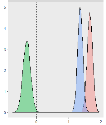
Posterior densities (and difference between…)

And, some more plots:

Finally, some model comparison:
priors <- c(prior(normal(0, 1.5), class = Intercept),
            prior(normal(0, 1.5), class = b),
            prior(exponential(5), class = sd))

m_null <-  brm(correct ~ loc + I(loc^2) +
                 (loc + I(loc^2)  |participant),
               data = d,
               prior = priors,
               family = "bernoulli")





model_weights(m_full, m_null)

    m_full       m_null 
0.0001219223 0.9998780777 

We get some low ESS warnings here, but I’m not too worried about this at present. Maybe I am wrong about this, but I’d rather work out what I want to be going, before polishing things.

EDIT by Aki: fixed summary output formatting

[Alasdair_Clarke]

Hello,

sorry for chasing on this but my co-authors are keen for my advice and I’m still not really sure what to suggest.

Any ideas?

To recap.. . I am looking for a good criterion for deciding an effect is present, so that we can then do a simulation-based “power” analysis.

This may likely be used in the actual experiment, as they are keen to use some stopping rule procedure for determining when to end data collection.

Thanks again

[p-lex]

My understanding is that you’ve calculated the probability of direction (“probability that the green distribution is <0”) which actually does not translate into “this effect is unlikely to be 0” but “the effect has a probability of … of being negative” (see Reporting Guidelines • bayestestR ). As you suggested, you could compare models and potentially use Bayes Factors to quantify the evidence (see Chapter 13 Bayes factors | Introduction to Bayesian Data Analysis for Cognitive Science or the published paper Workflow techniques for the robust use of bayes factors - PubMed ). There is also some info about power analysis in that chapter:

The Wang and Gelfand (2002) approach is as follows. We have adapted the procedure outlined below slightly for our purposes, but the essential ideas are due to these authors.

1. Decide on a distribution for the effect sizes you wish to detect.
2. Choose a criterion that counts as a threshold for a decision. This can be a Bayes factor of, say, 10 (Jeffreys 1939).⁵¹
3. Then do the following for increasing sample sizes n:

   1. Simulate prior predictive data niter times (say, niter=100) for sample size n; use informative priors (these are referred to as sampling priors in Wang and Gelfand 2002).

   2. Fit the model to the simulated data using regularizing (or principled) priors (these are called fitting priors in Wang and Gelfand 2002), and derive the posterior distribution each time, and compute the Bayes factor using a null model that assumes a zero effect for the parameter of interest.

   3. Display, in one plot, the niter posterior distributions and the Bayes factors. If the chosen decision criterion is met reasonably well under repeated sampling for a given sample size, choose that sample size.

I’m rather new to this myself, so take my advice with a pinch of salt.

[jsocolar]

Correct me if I’m wrong, but it look like you’ve included an intercept in your null model and not your full model. Maybe this accounts for your loo result? If not, I’ll note that in your full model you are estimating coefficients for the interactions of condition with both loc and loc^2, and this could make predictions worse even if including the main effect of condition is making predictions better.

[avehtari]

• The participant specific varying terms seem to explain a lot, and as this is included in both full and null, and using the LOO-CV predictive performance is dominated by this part hiding everything else in performance comparison. Looking at the posterior is still valid (and no need for BF)
• If you want to use cross-validation to see better the effect of the population terms, it would be better to use leave-one-participant-out with joint log score. See K-Fold Cross-Validation — kfold.brmsfit • brms, and use group="participant" and joint=TRUE. If you have a very large number of participants, you can also use K=10, folds="grouped", group="participant" to reduce the number of refits to 10.
• I repeat that don’t use model_weights(m_full, m_null) for model comparison as it is meant for model averaging, and as I said it can have a weight near 1 for one model when the models have very similar predictive distributions.
• If looking at the posterior is not enough for you, and you want to look at the predictive performance, too, see Sections 13 and 15 in Nabiximols treatment efficiency, and especially in Section 15 how to drop out the aleatoric part from th predictive comparison (still better to use the leave-participants-out).