Hierarchical regression with repeated measures in both x and y AND missing data

seth_musker · December 20, 2025, 3:15pm

When both x and y are repeatedly measured and there is a group-level relationship between them and there is missing data, the default for brms results in a misspecified model (I think!).

make_data <- function(
    n_groups=20,
    n_per_group = 5,
    y_int_mean = 5,
    y_int_sd=.5,
    y_sigma = 0.35,
    x_coef=2.3,
    x_sigma=0.1,
    seed=1,
    miss_type = c("random","groupwise"),
    missingness = 0,
    output_type=c("full","pergroup"),
    plot=FALSE
){
  miss_type <- match.arg(miss_type,miss_type)
  output_type <- match.arg(output_type,output_type)
  set.seed(seed)
  n_groups <- 20
  y_int_mean <- 5
  y_int_sd <- 0.5
  y_int_groups <- rnorm(n_groups,0,y_int_sd)
  x_coef <- 2.3
  x_true <- runif(n_groups)
  y_true <- y_int_mean + y_int_groups + x_true*x_coef
  
  # Take repeated measurements of x_true and y
  n_per_group <- 5
  y_sigma <- 0.35
  y_obs <- unlist(sapply(y_true,\(i)rnorm(n_per_group,i,y_sigma),simplify = F))
  x_sigma <- 0.1
  x_obs <- unlist(sapply(x_true,\(i)rnorm(n_per_group,i,x_sigma),simplify = F))
  
  groups <- rep(1:n_groups,each=n_per_group)
  
  if(plot){
    plot(y_obs~x_obs,col=groups)
    abline(lm(y_obs~x_obs),lty=2)
    abline(a=y_int_mean,b=x_coef)
    legend(
      "topleft",
      legend = c("true relationship",paste0("this instance (seed = ",seed,")")),
      lty = c(1,2)
    )
  }
  
  ## Put it in a big data frame -------------------------------------------------
  
  dat <- tibble(
    groups = as.factor(groups),
    y_obs = y_obs,
    x_obs = x_obs,
    y_true = rep(y_true,each=n_per_group),
    x_true = rep(x_true,each=n_per_group)
  ) %>% 
    group_by(groups) %>% 
    mutate(
      y_obs_mean_per_group = mean(y_obs),
      x_obs_mean_per_group = mean(x_obs)
    ) %>% 
    ungroup()
  
  ### Add missing values ----------------------------------------------------
  if(miss_type=="random") {
    assertthat::assert_that(missingness>=0 && missingness < 1)
    mis <- if_else(!rbinom((n_groups*n_per_group),1,missingness),1,NA)
    dat <- dat %>% 
      mutate(x_obs = x_obs*mis)
  } else {
    is.whole <- function(x, tol = .Machine$double.eps^0.5) abs(x - round(x)) < tol
    assertthat::assert_that(is.whole(missingness))
    mis <- sample(unique(dat$groups),size = missingness)
    dat <- dat %>% 
      mutate(x_obs = if_else(groups %in% mis,NA,x_obs))
  }
  
  attr(dat,"true_intercept") <- y_int_mean
  attr(dat,"true_slope") <- x_coef
  
  if(output_type == "full"){
    return(dat)
  } else {
    return(
      dat %>% 
        drop_na() %>% 
        group_by(groups) %>% 
        filter(n()>1) %>% 
        summarise(
          y_obs1=mean(y_obs),
          x_obs1=mean(x_obs),
          n=n(),
          sd_y=sd(y_obs),
          se_y=sd_y/sqrt(n-1),
          sd_x=sd(x_obs),
          se_x=sd_x/sqrt(n-1)
        ) %>% 
        rename(y_obs = y_obs1, x_obs = x_obs1)
    )
  }
}

library(tidyverse)
library(brms)
options("brms.backend" = "cmdstanr")
library(marginaleffects)
library(tidybayes)

dlist <- lapply(1:10,\(x) make_data(seed=x,missingness = .3))


# set_rescor(FALSE): Default brms behaviour ----------------------------------

bf_no_rescor <- bf(y_obs ~ mi(x_obs) + (1 | groups)) +
  bf(x_obs | mi() ~ 1 + (1 | groups)) 
bmer_no_rescor <- brm_multiple(
  bf_no_rescor,
  data = dlist,
  prior = c(
    prior(student_t(3,0,2.5),class=b,resp=yobs)
  ),
  seed=1L,
  chains=4,
  cores=4,
  iter=2000,
  combine = FALSE
)
bmer_no_rescor[[1]]

p1 <- lapply(
  bmer_no_rescor,
  \(x) plot_predictions(
    x,
    condition = "x_obs",
    re_formula = NA,
    resp = "yobs",
    draw = F
  )
) %>% 
  bind_rows(.id="Model") %>% 
  ggplot()+
  geom_abline(
    intercept = attributes(dlist[[1]])$true_intercept,
    slope = attributes(dlist[[1]])$true_slope
  )+
  geom_lineribbon(
    aes(x=x_obs,y=estimate,ymin=conf.low,ymax=conf.high,colour=Model,fill=Model),
    alpha=0.4
  )+
  facet_wrap(vars(Model))+
  theme_minimal()+
  labs(title="Model with set_rescor(FALSE) [default behaviour]")


#  set_rescor(TRUE) --------------------------------------------------

bf_rescor <- bf(y_obs ~ mi(x_obs) + (1 | groups)) +
  bf(x_obs | mi() ~ 1 + (1 | groups)) +
  set_rescor(TRUE)
bmer_rescor <- brm_multiple(
  bf_rescor,
  data = dlist,
  prior = c(
    prior(student_t(3,0,2.5),class=b,resp=yobs)
  ),
  seed=1L,
  chains=4,
  cores=4,
  iter=2000,
  combine = FALSE
)
bmer_rescor[[1]]

p2 <- lapply(
  bmer_rescor,
  \(x) plot_predictions(
    x,
    condition = "x_obs",
    re_formula = NA,
    resp = "yobs",
    draw = F
  )
) %>% 
  bind_rows(.id="Model") %>% 
  ggplot()+
  geom_abline(
    intercept = attributes(dlist[[1]])$true_intercept,
    slope = attributes(dlist[[1]])$true_slope
  )+
  geom_lineribbon(
    aes(x=x_obs,y=estimate,ymin=conf.low,ymax=conf.high,colour=Model,fill=Model),
    alpha=0.4
  )+
  facet_wrap(vars(Model))+
  theme_minimal()+
  labs(title="Model with set_rescor(TRUE) [non-default behaviour]")

patchwork::wrap_plots(p1,p2,guides = "collect")

Output of the code:

bmer_no_rescor[[1]]
Family: MV(gaussian, gaussian) 
  Links: mu = identity
         mu = identity 
Formula: y_obs ~ mi(x_obs) + (1 | groups) 
         x_obs | mi() ~ 1 + (1 | groups) 
   Data: data[[i]] (Number of observations: 100) 
  Draws: 4 chains, each with iter = 2000; warmup = 1000; thin = 1;
         total post-warmup draws = 4000

Multilevel Hyperparameters:
~groups (Number of levels: 20) 
                   Estimate Est.Error l-95% CI u-95% CI Rhat Bulk_ESS Tail_ESS
sd(yobs_Intercept)     0.63      0.15     0.37     0.96 1.01      660      954
sd(xobs_Intercept)     0.27      0.06     0.18     0.41 1.01      603     1193

Regression Coefficients:
               Estimate Est.Error l-95% CI u-95% CI Rhat Bulk_ESS Tail_ESS
yobs_Intercept     5.99      0.24     5.55     6.46 1.01      896     1622
xobs_Intercept     0.51      0.06     0.38     0.63 1.00      847     1444
yobs_mix_obs       0.64      0.38    -0.11     1.39 1.01      808     1090

Further Distributional Parameters:
           Estimate Est.Error l-95% CI u-95% CI Rhat Bulk_ESS Tail_ESS
sigma_yobs     0.30      0.02     0.26     0.35 1.00     3104     3079
sigma_xobs     0.11      0.01     0.09     0.14 1.00     1599     2389

bmer_rescor[[1]]
Family: MV(gaussian, gaussian) 
  Links: mu = identity
         mu = identity 
Formula: y_obs ~ mi(x_obs) + (1 | groups) 
         x_obs | mi() ~ 1 + (1 | groups) 
   Data: data[[i]] (Number of observations: 100) 
  Draws: 4 chains, each with iter = 2000; warmup = 1000; thin = 1;
         total post-warmup draws = 4000

Multilevel Hyperparameters:
~groups (Number of levels: 20) 
                   Estimate Est.Error l-95% CI u-95% CI Rhat Bulk_ESS Tail_ESS
sd(yobs_Intercept)     0.37      0.10     0.20     0.60 1.00      861     1469
sd(xobs_Intercept)     0.31      0.07     0.20     0.46 1.00     1100     1463

Regression Coefficients:
               Estimate Est.Error l-95% CI u-95% CI Rhat Bulk_ESS Tail_ESS
yobs_Intercept     5.31      0.20     4.88     5.70 1.00     1583     1690
xobs_Intercept     0.48      0.07     0.33     0.62 1.00      823     1341
yobs_mix_obs       2.06      0.36     1.36     2.79 1.00     1289     1570

Further Distributional Parameters:
           Estimate Est.Error l-95% CI u-95% CI Rhat Bulk_ESS Tail_ESS
sigma_yobs     0.37      0.04     0.30     0.47 1.00     1229     1915
sigma_xobs     0.11      0.01     0.09     0.14 1.00     1984     2475

Residual Correlations: 
                  Estimate Est.Error l-95% CI u-95% CI Rhat Bulk_ESS Tail_ESS
rescor(yobs,xobs)    -0.57      0.12    -0.76    -0.30 1.00     1380     2501

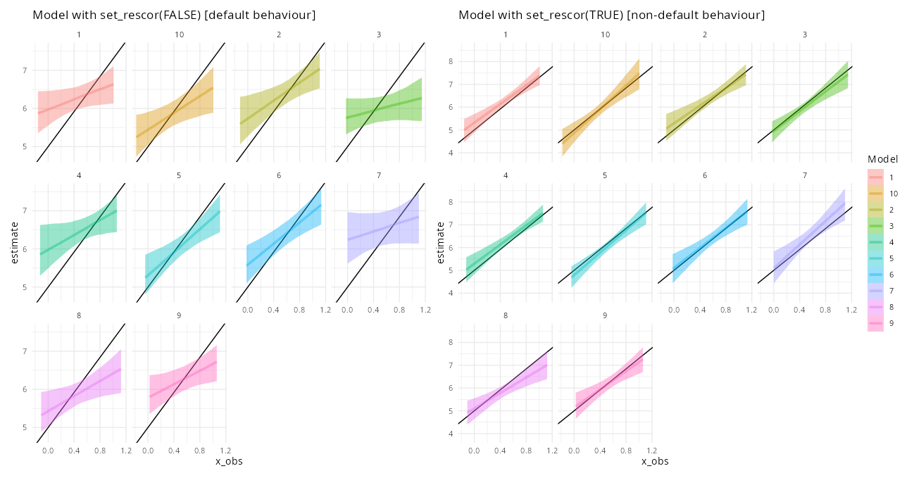
Edit: in the plot the legend title should really be “Data replicate”.

Could someone explain what’s going on here? Why is the rescor element so important? And is the first model actually not misspecified, but instead somehow appropriate given the simulation? Sorry, I’m about to get on a plane so I don’t have time to write a more considered post.

Operating System: Mint 22.2
brms Version: 2.23.0

hansvancalster · December 24, 2025, 1:58pm

I think that the way you simulate the data includes measurement error in the predictor variable:

This might explain why you see shallower slopes in the “default model without residual correlation” (attenuation bias). Adding the residual correlations will jointly model (y, x), which makes it somewhat similar to what measurement error models do to correct for the attenuation bias (for instance orthogonal regression or major axis regression).

Topic		Replies	Views
Brms: Estimating residual correlation between two variables with measurement error brms fitting-issues , specification , multivariate-normal , brms	1	400	December 11, 2023
Multiple correlation structures in hierarchical models using brms brms	2	1925	March 5, 2020
Brms and heterogeneous residual covariance - equivalent of "at.level" function brms	4	1007	October 11, 2024
Problems fitting multivariate model with option set_rescor brms brms	4	111	June 17, 2025
Issue with mi() and residual correlations brms	6	451	May 17, 2019

Hierarchical regression with repeated measures in both x and y AND missing data

Related topics