Here is a simpler model that mimics the problem and behavior. Let’s assume
X_i \sim {\rm{Poisson}} \left( R_i \right)
and that rate R_i is modelled as
R_i={\rm{exp}} \left( m+Y_i\right),
where m is the mean log rate parameter and Y_i is a (random) effect of each observation i. Let’s further assume that these effects are temporally autocorrelated with AR1, such that
{\bf{Y}} \sim {\rm{MVN}}\left( {[0,0,...,0]^\rm{T} ,\Sigma } \right),
where
\Sigma = \left[ {\begin{array}{*{20}{c}} {{\sigma ^2}}&{\rho {\sigma ^2}}&{...}&{{\rho ^{n - 1}}{\sigma ^2}}\\ {\rho {\sigma ^2}}&{{\sigma ^2}}&{...}&{{\rho ^{n - 2}}{\sigma ^2}}\\ \vdots & \vdots & \ddots & \vdots \\ {{\rho ^{n - 1}}{\sigma ^2}}&{{\rho ^{n - 2}}{\sigma ^2}}&{...}&{{\sigma ^2}} \end{array}} \right]
which can be rewritten as conditional distributions of one time step given the previous as
{Y_i} \sim \left\{ {\begin{array}{*{20}{c}} {{\rm{Normal}}\left( {0,\sigma } \right){\rm{ if }}i = 1}\\ {{\rm{Normal}}\left( {\rho {Y_{i - 1}},\sigma \sqrt {1 - {\rho ^2}} } \right){\rm{ if }}i > 1} \end{array}} \right.
Here is some R code to generate data from the model
n=100 # number of time steps
rho=.5 # AC
sig=2 #standard deviation
m=1 #mean log rate


Y=as.vector(rep(0,n))
for (t in 1:n){

  if(t==1){
    Y[t]=rnorm(1,0,sig)

  }else{
    Y[t]=rnorm(1,rho*Y[t-1],sig*sqrt(1-rho^2))

  }

}

R=exp(Y+m)

X=rpois(n=n,lambda=R)
Here is some stan code to fit the model
data {
  int<lower=0> n;
  int X[n];
}


parameters {
  real Y_raw[n];

  real log_sig;
  real m;
  real logit_rho;

}
transformed parameters{
  real R[n];
  real Y[n];
  real<lower=0,upper =1> rho=inv_logit(logit_rho);
  real<lower=0> sig=exp(log_sig);

  for (i in 1: n){
    if (i == 1){
      Y[i]=Y_raw[i] * sig;
    }else{
      Y[i] = rho*Y[i-1]  + Y_raw[i] * sqrt(1-rho^2) *sig;

    }
    R[i]=exp(Y[i]+m);
  }

}

model {

  for(i in 1:n){
    Y_raw[i]~normal(0,1);
    X[i]~poisson(R[i]);

  }
  rho~beta(1,1);
  sig ~ cauchy(0,2.5);
  m ~ normal(0,5);
  target += log_inv_logit(logit_rho) + log1m_inv_logit(logit_rho);
  target += log_sig;
}
The transformation Y[i] = rho*Y[i-1] + Y_raw[i] * sqrt(1-rho^2) *sig is based on a very useful suggestion by @bbbales2 here Reparameterization of correlation parameter for improved computation? - #2 by bbbales2, and using the logit- and log-transforms for rho and sig tends to avoid problematic sharp drops in the posteriors of these parameters.
If I use n=100 as above, \bf{Y} looks something like this:
and estimating parameters in Stan successfully retrieves the parameters used for simulation (rho=0.5, m=1,sig=2):
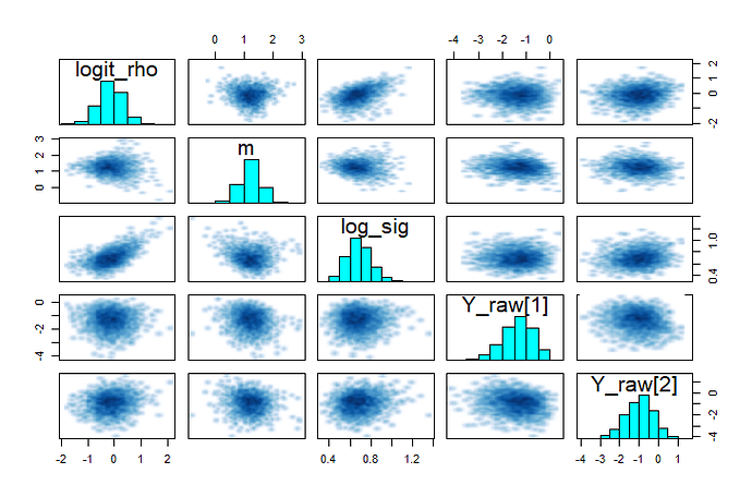
The pairs plots show some funnel behavior for m, but not too bad:
If I however reduce to n=15, the funnel behavior is augmented and the divergent transitions start showing their ugly faces:
Hopefully this better illustrates the nature of my problem. Just like in the original (real) example, the divergent transitions do not show up in the narrow part of the funnel, but my (admittedly limited) understanding from this post: Getting the location + gradients of divergences (not of iteration starting points) is that they don’t always appear where the problems arise. Suggestions for reparameterizations or other solutions that might work?


