Help with my divergent transitions, part 999

[tomli]

I’m working on a model with fairly many parameters (>5000) and is approaching 1000 lines of code, so I won’t attempt to get input on the entire thing, but I believe I have found some candidate parameters that might be causing my current problems with divergence, plotted as pairs below. The analysis is temporal, and each time iy has a parameter u[t], which is the autocorrelated temporal effect on “the thing this is modeling.” There are currently 11 time steps (NrOfYears) in the model.
logSu is the logarithm of standard deviation, Su, of u
logit_rhou is the logit-transform of first order autocorrelation rhou (I have for now excluded negative AC)
umean is the average parameter that u are distributed around
u_raw[1],u_raw[2] are examples the transformed parameters u on which they are updated.

I’m pasting in the code involving these parameters below in the hope that it might be sufficient to understand how they are modeled. One apparent issue is the funnel behavior umean. If that occur for the effects x around the mean, it often works to x[i]=x_raw[i] * sigma and x_raw[i] ~ normal(0, 1), but here it’s the mean that has a funnel behavior. Any idea of how to transform meanu to escape the funnel? I also think the correlation between logSu and `logit_rhou could be problematic.

In the plot, the blob of red dots are all from the same chain where almost all iterations diverged.

Grateful for any input.

Transformed parameters

rhou=inv_logit(logit_rhou);
Su=exp(logSu);

  for (iy in 1:NrOfYears){
    if (iy == 1){
      u[iy]=u_raw[iy] * Su;
    }else{
      u[iy] = rhou*u[iy-1]  + u_raw[iy] * sqrt(1-rhou^2) *Su;
    }
    
  }
  for (il in 1:NrOfLans){
    for (iy in 1:NrOfYears){
     
      loga[il,iy] = umean + u[iy]+v[il]; //the part of the model involving v appears to behave better
      a[il,iy] = exp (loga[il,iy] );
      
    }
  }

Model

  rhou~beta(1,1);
target += log_inv_logit(logit_rhou) + log1m_inv_logit(logit_rhou);

  for (iy in 1:NrOfYears){
   
    u_raw[iy] ~ normal(0, 1);
    
    //
    
    
  }


Su ~ cauchy(0,2.5);
  target += logSu;

[tomli]

Here is a simpler model that mimics the problem and behavior. Let’s assume

X_i \sim {\rm{Poisson}} \left( R_i \right)

and that rate R_i is modelled as

R_i={\rm{exp}} \left( m+Y_i\right),

where m is the mean log rate parameter and Y_i is a (random) effect of each observation i. Let’s further assume that these effects are temporally autocorrelated with AR1, such that

{\bf{Y}} \sim {\rm{MVN}}\left( {[0,0,...,0]^\rm{T} ,\Sigma } \right),

where

\Sigma = \left[ {\begin{array}{*{20}{c}} {{\sigma ^2}}&{\rho {\sigma ^2}}&{...}&{{\rho ^{n - 1}}{\sigma ^2}}\\ {\rho {\sigma ^2}}&{{\sigma ^2}}&{...}&{{\rho ^{n - 2}}{\sigma ^2}}\\ \vdots & \vdots & \ddots & \vdots \\ {{\rho ^{n - 1}}{\sigma ^2}}&{{\rho ^{n - 2}}{\sigma ^2}}&{...}&{{\sigma ^2}} \end{array}} \right]

which can be rewritten as conditional distributions of one time step given the previous as

{Y_i} \sim \left\{ {\begin{array}{*{20}{c}} {{\rm{Normal}}\left( {0,\sigma } \right){\rm{ if }}i = 1}\\ {{\rm{Normal}}\left( {\rho {Y_{i - 1}},\sigma \sqrt {1 - {\rho ^2}} } \right){\rm{ if }}i > 1} \end{array}} \right.

Here is some R code to generate data from the model

n=100 # number of time steps
rho=.5 # AC
sig=2 #standard deviation
m=1 #mean log rate


Y=as.vector(rep(0,n))
for (t in 1:n){
  
  if(t==1){
    Y[t]=rnorm(1,0,sig)
    
  }else{
    Y[t]=rnorm(1,rho*Y[t-1],sig*sqrt(1-rho^2))
    
  }
  
}

R=exp(Y+m)

X=rpois(n=n,lambda=R)

Here is some stan code to fit the model

data {
  int<lower=0> n;
  int X[n];
}


parameters {
  real Y_raw[n];
  
  real log_sig;
  real m;
  real logit_rho;
  
}
transformed parameters{
  real R[n];
  real Y[n];
  real<lower=0,upper =1> rho=inv_logit(logit_rho);
  real<lower=0> sig=exp(log_sig);
  
  for (i in 1: n){
    if (i == 1){
      Y[i]=Y_raw[i] * sig;
    }else{
      Y[i] = rho*Y[i-1]  + Y_raw[i] * sqrt(1-rho^2) *sig;
      
    }
    R[i]=exp(Y[i]+m);
  }
  
}

model {
  
  for(i in 1:n){
    Y_raw[i]~normal(0,1);
    X[i]~poisson(R[i]);
    
  }
  rho~beta(1,1);
  sig ~ cauchy(0,2.5);
  m ~ normal(0,5);
  target += log_inv_logit(logit_rho) + log1m_inv_logit(logit_rho);
  target += log_sig;
}

The transformation Y[i] = rho*Y[i-1] + Y_raw[i] * sqrt(1-rho^2) *sig is based on a very useful suggestion by @bbbales2 here Reparameterization of correlation parameter for improved computation? - #2 by bbbales2, and using the logit- and log-transforms for rho and sig tends to avoid problematic sharp drops in the posteriors of these parameters.

If I use n=100 as above, \bf{Y} looks something like this:

and estimating parameters in Stan successfully retrieves the parameters used for simulation (rho=0.5, m=1,sig=2):

The pairs plots show some funnel behavior for m, but not too bad:

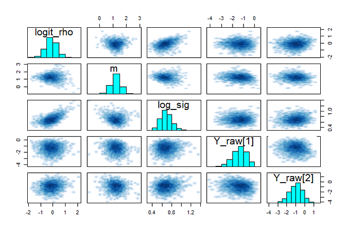
If I however reduce to n=15, the funnel behavior is augmented and the divergent transitions start showing their ugly faces:

Hopefully this better illustrates the nature of my problem. Just like in the original (real) example, the divergent transitions do not show up in the narrow part of the funnel, but my (admittedly limited) understanding from this post: Getting the location + gradients of divergences (not of iteration starting points) is that they don’t always appear where the problems arise. Suggestions for reparameterizations or other solutions that might work?

[martinmodrak]

Hi,
posting a simpler model is always a good idea :-) A quick look at the pairs plot suggests that the main issue is between m and log_sig where you either have low noise and m pretty well determined or high noise and m mostly undetermernied. This reminds of the Underdetermined Linear Regression case study. That could mean that for n=15 you just don’t have enough data to constrain the parameters very well and you either need to add prior information to avoid the low noise part of the posterior or add more data. I don’t think anybody is aware of a good reparametrization that would let you get rid of this issue. We also very briefly discuss it in section 5.10 of the Bayesian Workflow preprint.

[mike-lawrence]

Try a prior for the noise term that’s not peaked at zero. While standard, I find they usually reflect ridiculous beliefs. I like weibull(2,1) instead. Be sure to report back if that helps at all; I’d love to have a concrete example to advocate for a change in the prior recommendations.

[tomli]

Thanks Martin.
Here are pairs plots from simulations with rho=0.95, indicating that there are also some issues with that parameter when correlation is high. Though the funnel behavior observed in the pairs of m and logit_rho may very well be an indirect effect via the correlation between logit_rho and log_sigma.

[tomli]

Thanks Mike

Adding a different prior is likely a good idea. The Half-Cauchy I’ve implemented here isn’t peaked at zero. It’s plateau-shaped near zero while having a fat tail (all moments are infinite, if I remember correctly) that allows for really large values, should the data tell me so. Yet, the scale of 2.5, which was suggested by Gelman et al in some paper, admittedly doesn’t really really capture my prior beliefs about the system. A standard deviation of 2.5 (the scale is, if I’m not mistaken, the median of the Half-Cauchy) of effects is a massive difference for a model on the log scale. For the actual problem, I would prefer a prior that says “I think these time step effects are likely very small, but, hey, let’s allow the data to convince me otherwise if it’s strong enough.” Not sure what distribution and parameterization adheres to that notion. Maybe Half-Cauchy with a lower scale parameter, but that requires motivating that lower value.

What’s the motivation for using the Weibull? With the shape parameter >1, it has a sub-exponential tail, which is great for fitting but sounds hard to justify. I ran a few version of my toy example with Weibull(2,1), but it didn’t change much in terms of divergence. Her is an example of pairs

[mike-lawrence]

@tomli

The Half-Cauchy I’ve implemented here isn’t peaked at zero.

Looks pretty peaked-at-zero to me:

@tomli

What’s the motivation for using the Weibull? With the shape parameter >1, it has a sub-exponential tail, which is great for fitting but sounds hard to justify. I ran a few version of my toy example with Weibull(2,1), but it didn’t change much in terms of divergence. Her is an example of pairs

It’s just a shape I’ve found and like.

Peaked around .8, zero at zero, and only ~2% of mass above 2. If the data is scaled to have an empirical SD of 1, it makes for a broad but reasonable prior IMO.

@tomli

I ran a few version of my toy example with Weibull(2,1), but it didn’t change much in terms of divergence.

Ah, darn.

[tomli]

If the data is scaled to have an empirical SD of 1, it makes for a broad but reasonable prior IMO.

Gotcha. That approach sadly isn’t possible for neither the toy example (scaling count data isn’t straightforward) nor the real model I’m struggling with, where umean is the average log shape parameter of the Dirichlet distribution, so it’s already something scale free.

[mike-lawrence]

@tomli

scaling count data isn’t straightforward

Oh, sorry! I failed to notice you’re dealing with count data.

[martinmodrak]

To me this pairs plot looks quite typical of the “underdetermined regression” type. I can imagine (but that’s speculation) the rho parameter has partly similar effect to sigma - you either can have almost no correlation and then m is very tightly constrained (as if I understand the model right, in this case all Y should be almost equal to m so all observations directly inform m). This is however probably technically more challenging to avoid as you would actually need a bimodal prior to avoid values close to zero, which is likely to lead to all sorts of problems and is also likely not very justifiable (unlike saying “noise is > 0”, which is usually well justified).

@tomli

What’s the motivation for using the Weibull? With the shape parameter >1, it has a sub-exponential tail, which is great for fitting but sounds hard to justify. I ran a few version of my toy example with Weibull(2,1), but it didn’t change much in terms of divergence.

People have also used inverse gamma for similar purposes. In any case, the idea is that you just find parameters for the distribution so that e.g. 5% and 95% quantiles match your prior expectations about the range of the value. For this particular case you also want the tail towards zero to be very light (which AFAIK inverse gamma gives you). Ben Goodrich had a nice presentation on actually building custom priors directly from quantiles avoiding to choose the specific family (which tends to be quite arbitrary). https://www.youtube.com/watch?v=_wfZSvasLFk but that’s just an aside and is probably an overkill here.

In any case, I think the main problem is most likely that with low n you just can’t learn much about the parameters of your model and while adding prior info could help convergence, it is unlikely to remedy this problem.