I am trying to work out the best way to graph posterior predictive distributions from factorial models. I have created an example to highlight my issues
The data we will be modelling will be a mixed design, with both within- and between-subject factors. Each individual gets three conditions, but there are three between-subjects groups as well. There should be differences across condition (cond1 = 100, cond2 = 75, cond3 = 125), but not across groups. So no main effect of group, no main effect of condition, and no interaction
df <- data.frame(id = factor(rep(1:60, 3)),
                 group = factor(rep(c("g1", "g2", "g3"), each = 20, length.out = 180)),
                 condition = factor(rep(c("cond1", "cond2", "cond3"), each = 60)),
                 score = c(ceiling(rnorm(60, 100, 15)), ceiling(rnorm(60, 75, 15)), ceiling(rnorm(60, 125, 15))))
Graph it
ggplot(df) +
           geom_point(aes(x = condition, y = score, colour = group), shape = 1, position =   position_dodge(width=0.9)) +
           geom_boxplot(aes(x = condition, y = score, colour = group), alpha = 0, position = position_dodge(width=0.9)) +
           scale_colour_manual(values = c("#00AFBB", "#E7B800", "#616a6b"))
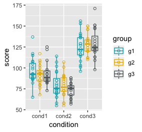
We can see the differences across conditions and absence of difference between groups. Now to run the model and sample from the posterior via the generated quantities block.
##### Step 1: put data into a list
mixList <- list(N = nrow(df),
                nSubj = nlevels(df$id),
                nGroup = nlevels(df$group),
                nCond = nlevels(df$condition),
                nGxC = nlevels(df$group)*nlevels(df$condition),
                sIndex = as.integer(df$id),
                gIndex = as.integer(df$group),
                cIndex = as.integer(df$condition),
                score = df$score,
                grandMean = 102.0056,
                stdDev = 25.81834) # from mean of score averaged across groups and conditions


###### Step 2: build model
write("
    data{
    int<lower=1> N;
    int<lower=1> nSubj;
    int<lower=1> nGroup;
    int<lower=1> nCond;
    int<lower=1,upper=nSubj> sIndex[N];
    int<lower=1,upper=nGroup> gIndex[N];
    int<lower=1,upper=nCond> cIndex[N];
    real score[N];
    real grandMean;
    real stdDev;
    }

    parameters{
    real a;
    vector[nSubj] bSubj;
    vector[nGroup] bGroup;
    vector[nCond] bCond;
    vector[nCond] bGxC[nGroup];      // vector of vectors, stan no good with matrix
    real<lower=0> sigma;
    real<lower=0> sigma_a;
    real<lower=0> sigma_s;
    real<lower=0> sigma_g;
    real<lower=0> sigma_c;
    real<lower=0> sigma_gc;
    }

    model{
    vector[N] mu;

    //hyper-priors
    sigma_s ~ normal(0,10);
    sigma_g ~ normal(0,10);
    sigma_c ~ normal(0,10);
    sigma_gc ~ normal(0,10);


    //priors
    sigma ~ cauchy(0,2);
    a ~ normal(grandMean, stdDev);
    bSubj ~ normal(0, sigma_s);
    bGroup ~ normal(0,sigma_g);
    bCond ~ normal(0,sigma_c);
    for (i in 1:nGroup) {               //hierarchical prior on interaction
    bGxC[i] ~ normal(0, sigma_gc);
    }

    // likelihood
    for (i in 1:N){
    mu[i] = a + bGroup[gIndex[i]] + bCond[cIndex[i]] + bSubj[sIndex[i]] + bGxC[gIndex[i]][cIndex[i]];
    }
    score ~ normal(mu, sigma);
    }

    generated quantities{
    real y_draw [N];

    for (i in 1:N) {
    y_draw[i] = normal_rng(a + bGroup[gIndex[i]] + bCond[cIndex[i]] + bSubj[sIndex[i]] + bGxC[gIndex[i]][cIndex[i]],sigma);
    }
    }
    ", file = "temp.stan")

##### Step 3: generate the chains
mixInt0_noMatrix_hyper <-  stan(file = "temp.stan",
                                data = mixList,
                                iter = 2.1e4,  # 20,000 estimates
                                warmup = 1e3,   # 1000 warmups
                                cores = 1,
                                chains = 1)
Now we extract the draws from the joint posterior distribution.
y_draw <- as.matrix(mixInt0_noMatrix_hyper, pars = "y_draw")
This will give us a 20000 x 180 matrix, with 20000 draws from the posterior for each data point in the original. Now I have to confess I couldn’t think of another way to do this. Ideally I would like to drawl marginal main effects of group and condition as well as marginal interaction effects for the model but instead I have a column for each data point. All I could think to do was take the mean of the 20000 posterior draws
drawMu <- apply(y_draw, 2, mean)
Then pass those mean draws into the original dataframe
df$draw <- drawMu
And graph the mean posterior draws against the original data. In this graph the points are the actual data points and the boxplots are the mean draws from the posterior for each data point.
ggplot(df) +
           geom_point(aes(x = condition, y = score, colour = group), shape = 1, position = position_dodge(width=0.9)) +
           geom_boxplot(aes(x = condition, y = draw, colour = group), alpha = 0, position = position_dodge(width=0.9)) +
           scale_colour_manual(values = c("#00AFBB", "#E7B800", "#616a6b"))

It looks like the model has retrieved the the overall pattern of cell means within the model quite well but the boxplots are far too small, with far too little uncertainty in the estimates. I would really like to do all of this much better. For instance it might be nice to graph differences in conditions averaged across groups, or in groups averaged across conditions using these draws from the posterior.
Can anyone suggest how best to graph posterior predictive distributions for this sort of grouped mixed factorial model?