Gaussian model performs better despite worse fit

[neurotroph]

Hey there!

I’m trying to model preferred prices and have quickly set up a simple linear model. The Gaussian model makes worse predictions on a case-by-case basis, but the average predictions match the data pretty well. When a use a more appropriate GLM, that has better posterior predictive checks, the averaged predictions are way off.

Backstory: There are several features and users are able to select their preferred combination. Afterwards they enter a preferred price for the selected features. I have a dataset on those preferred prices. The problem is, that there is data missing for cases that have selected only one of the features. The datasets contains cases where the features has been included in a combination.
Furthermore, there is a preferred price for a similar service in the dataset, so I know each user’s general price preference (highly correlated with the preferred price for the selected features).

Using brms the simple Gaussian model looks like this:

df_train <- read_csv(...)
bm.gauss <- brm(PPrice_Combination <- Feature_1 + Feature_2 + Feature_3 + PPrice_Alternative, data = df_train, family = Gaussian())

Feature_1 through Feature_3 are 0/1-coded. PPrice_Combination and PPrice_Alternative are continuous, positive values.

Model converges and looks fine. Looking at the posterior predictive checks, the model obviously doesn’t fit very well:

Looking at the model’s posterior predictions, unsurprisingly, they don’t really make sense with a lot of negative values. When comparing the averaged predictions for each combination to the actual averages, the model performs pretty well, though:

Feature Selection	Actual Mean	Predicted Mean
1	144.06	144.06
1 + 2	309.62	309.62
1 + 2 + 3	362.18	362.18
1 + 3	589.25	589.25
2 + 3	516.41	516.41

Looks pretty overfit, but predictions for the missing features look very sensible:

Feature Selection	Actual Mean	Predicted Mean
2	-	37.77
3	-	216.72

Now, the model is obviously wrong, but useful. Since it would be interesting to have better predictions for individual users, I was looking for a better model. As all responses are positive, I was looking into a lognormal model:

bm.lognorm <- brm(PPrice_Combination <- Feature_1 + Feature_2 + Feature_3 + PPrice_Alternative, data = df_train, family = lognormal())

Comparing the model using WAIC favors the lognormal model and posterior predictive check looks better:

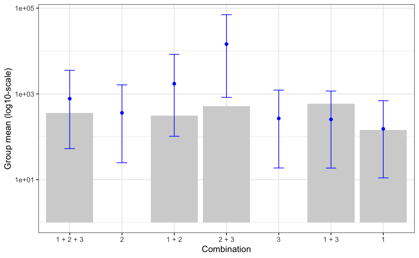
But predictions are pretty off:

Feature Selection	Actual Mean	Predicted Mean
1	144.06	94.81
1 + 2	309.62	1081.95
1 + 2 + 3	362.18	440.18
1 + 3	589.25	201.66
2 + 3	516.41	8680.69

So, despite being a better model, the predictions are not really as good so that I would put faith in them. It’s really interesting to see this go like this, but I was wondering what possible steps would be to improve the model and its predictions. I have tried using other models or transformations (such as log-transforming or standardising the responses), but model fit or prediction accuracy did not increase.

Any recommendations for a better approach?

Thanks!
Chris

[torkar]

Hi,

well, take this for what it is :)

0. Can you post original data, a subset of the data, or simulated data that fits your scenario?
1. Use lognormal as likelihood seems ok in your case.
2. Do you have lots of zeros in your outcome variable PPrice_Combination?
3. PPrice_Alternative should be standardized (the other Feature_n variables are 0/1 as you write so probably leave them be for now :)
4. Check your priors (what priors do you have?) Have you done prior predictive checks, i.e., something like this:
   a) After you’ve set \beta priors in brms
   b) run brms with sample_prior="only"
   c) run pp_check(ModelName) to check the fit.

[neurotroph]

Thanks, @torkar! Great starting point.

0. Can’t post original or subset of data, sorry. I have created a synthetic dataset using synthpop, but there are differences in model performance and prediction accuracy between the original and the synthetic data (link see below).
1. :)
2. No zeroes at all in the outcome.
3. I tried to standardize the predictor, but results are pretty much unchanged.
4. Yes, I was missing the prior specification in the brms snippet. For some naïve reason I thought that brms would use wide normal priors if no priors are specified. So, when adding weakly regularising priors (N(\mu = 0; \sigma = 100)) results are similar, though.

Looking at the posterior check posted above, I noticed that I pasted the wrong figure, unfortunately. The curve above is not from the log-normal model, but from a Gaussian model on the log-transformed response. That model was looking great in the posterior predictive checks but resulted in similarly wrong predictions.

For the log-normal model the posterior predictive checks are not easy to read, possibly due to outliers:

Comparing four different model specifications leads to the following plots:

I haven’t used prior predictive checks before. How would I interpret them correctly? Interestingly, I cannot plot the pp_check, because the predictions for the log-normal model are non-sensical:

> pp_check(bm.lognormal, type = "dens_overlay")
Using 10 posterior samples for ppc type 'dens_overlay' by default.
Error in if ((w[1] * sm + w[2] * cm + w[3] * dm + w[4]) < best$score) break : 
  missing value where TRUE/FALSE needed
> predict(bm.lognormal)
            Estimate Est.Error          Q2.5         Q97.5
  [1,] 3.809892e+222       Inf 5.252097e-137 2.818929e+132
  [2,]           Inf       NaN  0.000000e+00           Inf
  [3,]           Inf       NaN 3.661417e-219 1.377812e+212
  [4,] 1.427724e+171       Inf 1.714141e-107 5.274732e+102
  [5,]           Inf       NaN  0.000000e+00           Inf
  [6,] 3.896258e+171       Inf 1.885539e-111 2.616608e+110
  [7,] 1.021810e+207       Inf 1.826580e-126 5.786957e+123
# ...
> summary(bm.lognormal)
 Family: lognormal 
  Links: mu = identity; sigma = identity 
Formula: PPrice_Combination ~ Feature_1 + Feature_2 + Feature_3 + PPrice_Alternative1_std + PPrice_Alternative2_std
   Data: df_train_bayes (Number of observations: 406) 
Samples: 4 chains, each with iter = 2000; warmup = 1000; thin = 1;
         total post-warmup samples = 4000

Population-Level Effects: 
          Estimate Est.Error l-95% CI u-95% CI Rhat Bulk_ESS Tail_ESS
Intercept    -1.02    169.22  -345.58   332.69 1.00     6164     3176
Feature_1    -0.07    101.84  -201.42   201.08 1.00     6950     3212
Feature_2    -0.89     99.61  -195.84   194.68 1.00     6838     3033
Feature_3     1.15     97.66  -187.78   194.30 1.00     6456     3070
Alt1_std     -0.96     99.92  -198.82   194.07 1.00     6135     2797
Alt2_std     -1.85     98.55  -195.71   195.65 1.00     6340     2839

Family Specific Parameters: 
      Estimate Est.Error l-95% CI u-95% CI Rhat Bulk_ESS Tail_ESS
sigma    11.08     14.10     0.34    40.82 1.00     4406     2265

Samples were drawn using sampling(NUTS). For each parameter, Eff.Sample 
is a crude measure of effective sample size, and Rhat is the potential 
scale reduction factor on split chains (at convergence, Rhat = 1).

The problem doesn’t occur with the synthetic data, so not sure if that really helps. Nevertheless, I have uploaded everything to this Git repository: https://github.com/neurotroph/Pricing_GLM

Do you have further recommendations how to go from here?

Thanks & best regards
Christopher

[torkar]

In the data you have PPrice_Alternative1 and PPrice_Alternative2?

[neurotroph]

Yes, that’s correct. Sorry, in my initial post I talked only about a single price point, but actually we have two alternative products for which we have a preferred price. Both correlate strongly with the preferred price for the selected combination, so I’ve included both in the model as a baseline for preferred prices.

[torkar]

So enough to use one of them in the model for now? Also, the data has NAs:

> table(is.na(d))

FALSE  TRUE 
 2669   131

[torkar]

Here’s my try. Seems to work quite nicely :)

library(brms)
library(bayesplot)
library(ggplot2)

d <- read.csv("Data/PricingGLM_SynthData.csv", sep=",")

d$PPrice_Alternative1_s <- scale(d$PPrice_Alternative1)
d$PPrice_Alternative2_s <- scale(d$PPrice_Alternative2)
d$F1 <- d$Feature_1
d$F2 <- d$Feature_2
d$F3 <- d$Feature_3

p <- get_prior(PPrice_Combination ~ F1 + F2 + F3 +
                 PPrice_Alternative1_s,
               data = d, family = lognormal)

p$prior[1] <- "normal(0,1)"
p$prior[6] <- "normal(0,2.5)"
p$prior[7] <- "weibull(2,1)"

M_prio <- brm(PPrice_Combination ~ F1 + F2 + F3 + PPrice_Alternative1_s,
              prior = p, data = d, family = lognormal, sample_prior = "only")

pp_check(M_prio) + scale_x_continuous(trans = "log2")

M <- brm(PPrice_Combination ~ F1 + F2 + F3 + PPrice_Alternative1_s,
              prior = p, data = d, family = lognormal)

pp_check(M) + scale_x_continuous(trans = "log2")

Rplot.pdf (58.4 KB)

[neurotroph]

Thank you for your very constructive help, @torkar!

The NAs should only occur if Feature_1 == 0 & (Feature_2 == 1 XOR Feature_3 == 1), i.e. it’s those cases that I’m trying to predict. For fitting the model, I therefore use only the subsample of cases where PPrice_Combination is present: df %>% filter(!is.na(PPrice_Combination)).

D’oh, thanks for reminding me about scale_x_continuous(log = "log2"). That makes everything more readable. :) Yes, the log-normal posterior predictive check looks good and model seems to be a better fit based on this.

This, nonetheless, brings me back to my initial question, because the log-normal model still gives predictions that, when aggregated to a group mean, are implausible. Compared to the simple Gaussian model, that provides better aggregated predictions but gives implausible individual predictions.

Looking at the predictions from the log-normal model (blue) compared to the actual data (grey bars), shows that the 95% posterior interval isn’t looking so bad, but maximum a posteriori predictions for combinations “1+2” (458% relative deviation) and “2+3” (2,707% relative deviation) are off by orders of magnitude.

Somehow, it makes intuitive sense to me, that the Gaussian model performs well on means. I’m still wondering how I can further improve the log-normal model for better predictions – because it seems like there is more information available, that isn’t used yet (does this make sense?).

[torkar]

Hi,

how would a model look like with all predictors included?

Are you saying that the two PPrice_Alternative variables are what you use to calculate your PPrice_Combination, i.e., your outcome? (I would strongly recommend to skip missing data for now and incorporate that into the model once you have a better model to work with.)

Sorry… I have a hard time seeing what you want to accomplish but then I don’t have your domain knowledge :)