Dear Stan Users,
I hope this message finds you well.
I have been working on Gamma Spatial Generalized Linear Mixed Models (SGLMMs) using Eigenbasis spatial functions for the covariance matrix across 5000 locations. My goal is to compare the posterior estimates from my Metropolis-Hastings MCMC implementation with those from RStan, particularly via diagnostic and posterior plots.
I’ve attached the following:
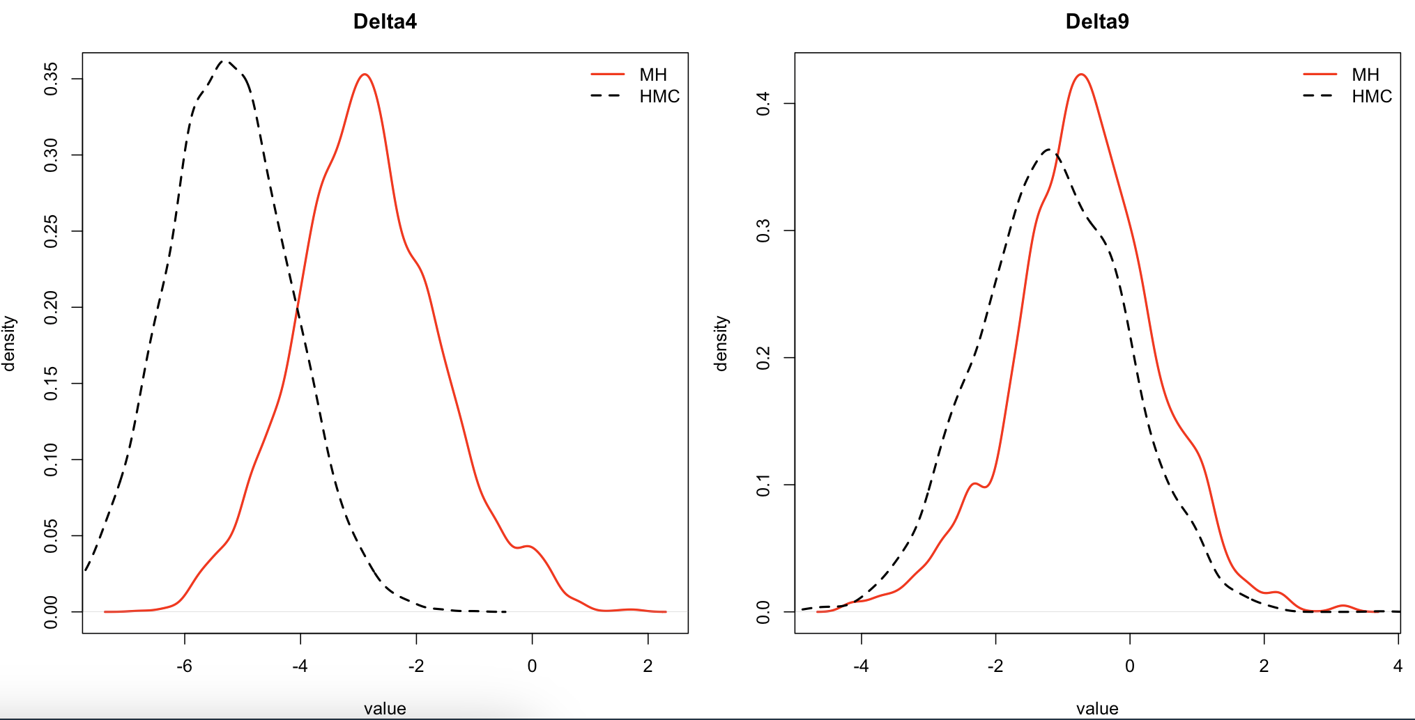
The plot below shows that the posterior for β looks reasonable, but the other parameters differ notably—especially log(σ²) and alpha. I suspect this discrepancy may be driving the overall difference, but I’m unsure why it’s happening.
Could you kindly review my RStan code to see if there are any issues? I guess my RStan code has some problems but I can’t figure out more than two weeks.
Thank you very much in advance for your time and help.
Best regards,
Best,
JH
A few thoughts:
You give logsigma2 a lower bound of 0, meaning that \sigma will never be less than 1. This could be driving differences in your deltas, though I’m not seeing why your \sigma^2 estimate is so large compared with the prior; it looks like the bulk of your posterior for it is greater than 25, which has a severe mismatch with the prior encoded in the model. Is there a chance there’s an error in the post-processing script when you made the posterior plot?
It might be worth considering changing the model to put a half-normal or half-t prior directly on \sigma.
The other thing I’ll note is that my may get some model improvement by reparameterizing your deltas to use a non-centered parameterization.
Original model for reference:
data {
  int N; // the number of observations
  int K; // the number of columns in the model matrix
  int P; // the number of columns in the basis matrix
  matrix[N, K] X; // the model matrix
  matrix[N, P] M; // the basis matrix
  real<lower=0> y[N]; // response (continuous positive values)
}

parameters {
  vector[K] betas; // the regression parameters
  vector[P] deltas; // the reparameterized random effects
  real<lower=0> logsigma2; // the variance parameter for sigma^2
  real<lower=0> alpha; // shape parameter for gamma
}

transformed parameters {
  vector[N] linpred;
  vector[N] mu; // the expected values (probabilities of success)
  // Linear predictor calculation
  linpred = X * betas + M * deltas;

  // Applying the log link function to get probabilities
  mu = exp(linpred);  ;
}

model {
  betas ~ normal(0, 10); // prior for betas
  logsigma2 ~ normal(0, 0.5); // prior for variance parameter
  deltas ~ normal(0, sqrt(exp(logsigma2))); // prior for the random effects
  alpha ~ gamma(5, 5); // prior for shape

  // Likelihood: Gamma distribution for continuous positive response
  y ~ gamma(alpha, mu);
}